Magnitude Frequency Distribution#
In seismic hazard analysis, magnitude frequency distribution (MFD) is one of the important parameter that must be considered. The MFD is used for estimating the number of earthquakes (occurrence rate) of each magnitude bin for a region of interest that follows the Gutenberg-Richter’s Law,
$$log_{10} N (\ge M) = a - bM_c$$
or
$$N (\ge M) = 10^{a - bM}$$
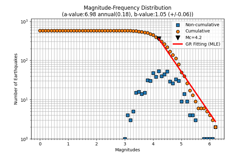
where the $N (\ge M)$ is the number of earthquakes that has magnitude greater than $M$, $M_c$ is the magnitude of completeness, $a$ and $b$ are the statistical seismicity parameters that describes the seismicity activity rate and small-large event ratio, respectively. The $b$ value has tipically value of 1 in global. The MFD data is estimated from earthquake catalog and it presents by two informations, non-cumulative and cumulative as shown in Figure 1 below.
For simple calculation illustration, assuming $a = 1$, $b = 1$ and $M_c = 0$, we can easy to calculate the number of earthquakes that greater than $M_c = 0$ by
$$log_{10} N (\ge M) = a - bM_c$$
$$log_{10} N (\ge M=0) = 1 - 1 * 0$$
$$log_{10} N (\ge M=0) = 1 - 0 = 1$$
$$N (\ge M=0) = 10^1 = 10$$
This calculation estimated 10 cumulative earthquakes that having magnitude greater than 0. Now, we try to change $M_c = 1$ and keep the same value for the rest of parameters.
$$log_{10} N (\ge M) = a - bM_c$$
$$log_{10} N (\ge M=1) = 1 - 1 * 1$$
$$log_{10} N (\ge M=1) = 1 - 1 = 0$$
$$N (\ge M=0) = 10^0 = 1$$
The number of earthquakes decreases by 10 times with increased the $M_c$. This information tells us that the events with large magnitude occur less frequently and lower occurrence rate comparing to the events that have low and medium magnitude. As illustrated in Figure 1 above, the number of earthquake of magnitude above 6 is about 3 events which is lower than the magnitude above 4 that has approximately about 400 events.
In the real case, the $b$ value can be calculated by using Maximum-Likelihood Estimation (MLE), proposed by Aki K, 1965 as written in Equation below
$$b = \frac {log_{10} e} {\bar M - M_c}$$
where $\bar M$ is mean of magnitude. Furthermore, the $a$ value can be calculated by using the GR’s Law as mentioned in equation above. We can also apply simple linear regression to calculate the $a$ and $b$ values. The $M_c$ is then estimated based on the higher frequency number of non-cumulative earthquake distribution. The $M_c$ becomes lower magnitude boundary for seismic hazard analysis.
This approach is suitable for region or area that has large seismicity distribution, such as subduction zone or background seismicity. For the seismicity around a fault, it is suggested to estimate the magnitude frequency distribution or occurrence rate by using Characteristic Earthquake Distribution, proposed by Youngs-Coppersmith, 1985.
The MFD calculation by using MLE and Gutenberg-Richter’s Law can be done by using seisliby.
References#
B. Gutenberg, C. F. Richter; Frequency of earthquakes in California. Bulletin of the Seismological Society of America 1944;; 34 (4): 185–188. doi: https://doi.org/10.1785/BSSA0340040185
Aki, K. (1965). 17. Maximum Likelihood Estimate of b in the Formula logN=a-bM and its Confidence Limits. 43(2), 237–239. https://repository.dl.itc.u-tokyo.ac.jp/records/33631
Robert R. Youngs, Kevin J. Coppersmith; Implications of fault slip rates and earthquake recurrence models to probabilistic seismic hazard estimates. Bulletin of the Seismological Society of America 1985;; 75 (4): 939–964. doi: https://doi.org/10.1785/BSSA0750040939