California Housing Prices

import kagglehub
import os
import pandas as pd
import seaborn as sns
import matplotlib.pyplot as plt
from matplotlib.ticker import MultipleLocator

path = kagglehub.dataset_download("camnugent/california-housing-prices")
file = os.listdir(path)[0]

Using Colab cache for faster access to the 'california-housing-prices' dataset.

About Dataset

https://www.kaggle.com/datasets/camnugent/california-housing-prices/data

Features

Feature’s Name	Information
longitude	A measure of how far west a house is; a higher value is farther west
latitude	A measure of how far north a house is; a higher value is farther north
housingMedianAge	Median age of a house within a block; a lower number is a newer building
totalRooms	Total number of rooms within a block
totalBedrooms	Total number of bedrooms within a block
population	Total number of people residing within a block
households	Total number of households, a group of people residing within a home unit, for a block
medianIncome	Median income for households within a block of houses (measured in tens of thousands of US Dollars)
medianHouseValue	Median house value for households within a block (measured in US Dollars)
oceanProximity	Location of the house w.r.t ocean/sea

Objectives

1. Creating a model for predicting the house pricing given some informations.

Important, the data must be cleaned.

Acknowledgements

This data was initially featured in the following paper: Pace, R. Kelley, and Ronald Barry. “Sparse spatial autoregressions.” Statistics & Probability Letters 33.3 (1997): 291-297.

This dataset is a modified version of the California Housing dataset available from: Luís Torgo’s page (University of Porto)

# Reading file
df = pd.read_csv("/".join([path,file]))
df.head()

	longitude	latitude	housing_median_age	total_rooms	total_bedrooms	population	households	median_income	median_house_value	ocean_proximity
0	-122.23	37.88	41.0	880.0	129.0	322.0	126.0	8.3252	452600.0	NEAR BAY
1	-122.22	37.86	21.0	7099.0	1106.0	2401.0	1138.0	8.3014	358500.0	NEAR BAY
2	-122.24	37.85	52.0	1467.0	190.0	496.0	177.0	7.2574	352100.0	NEAR BAY
3	-122.25	37.85	52.0	1274.0	235.0	558.0	219.0	5.6431	341300.0	NEAR BAY
4	-122.25	37.85	52.0	1627.0	280.0	565.0	259.0	3.8462	342200.0	NEAR BAY

df.describe()

	longitude	latitude	housing_median_age	total_rooms	total_bedrooms	population	households	median_income	median_house_value
count	20640.000000	20640.000000	20640.000000	20640.000000	20433.000000	20640.000000	20640.000000	20640.000000	20640.000000
mean	-119.569704	35.631861	28.639486	2635.763081	537.870553	1425.476744	499.539680	3.870671	206855.816909
std	2.003532	2.135952	12.585558	2181.615252	421.385070	1132.462122	382.329753	1.899822	115395.615874
min	-124.350000	32.540000	1.000000	2.000000	1.000000	3.000000	1.000000	0.499900	14999.000000
25%	-121.800000	33.930000	18.000000	1447.750000	296.000000	787.000000	280.000000	2.563400	119600.000000
50%	-118.490000	34.260000	29.000000	2127.000000	435.000000	1166.000000	409.000000	3.534800	179700.000000
75%	-118.010000	37.710000	37.000000	3148.000000	647.000000	1725.000000	605.000000	4.743250	264725.000000
max	-114.310000	41.950000	52.000000	39320.000000	6445.000000	35682.000000	6082.000000	15.000100	500001.000000

# Checking the features
df.info()

<class 'pandas.core.frame.DataFrame'>
RangeIndex: 20640 entries, 0 to 20639
Data columns (total 10 columns):
 #   Column              Non-Null Count  Dtype
---  ------              --------------  -----
 0   longitude           20640 non-null  float64
 1   latitude            20640 non-null  float64
 2   housing_median_age  20640 non-null  float64
 3   total_rooms         20640 non-null  float64
 4   total_bedrooms      20433 non-null  float64
 5   population          20640 non-null  float64
 6   households          20640 non-null  float64
 7   median_income       20640 non-null  float64
 8   median_house_value  20640 non-null  float64
 9   ocean_proximity     20640 non-null  object
dtypes: float64(9), object(1)
memory usage: 1.6+ MB

# Checking the missing values in the dataset
df.isnull().sum()

	0
longitude	0
latitude	0
housing_median_age	0
total_rooms	0
total_bedrooms	207
population	0
households	0
median_income	0
median_house_value	0
ocean_proximity	0

dtype: int64

# Filling the missing value
df['total_bedrooms'] = df['total_bedrooms'].fillna(df['total_bedrooms'].median())
df.isnull().sum()

	0
longitude	0
latitude	0
housing_median_age	0
total_rooms	0
total_bedrooms	0
population	0
households	0
median_income	0
median_house_value	0
ocean_proximity	0

dtype: int64

# Checking the outliers for numerical features
df_OnlyFloat = df.select_dtypes('float64')
df_OnlyFloatCols = df_OnlyFloat.columns

fig, ax = plt.subplots(figsize=(10,8), ncols=3, nrows=3)
k = 0
for i in range(3):
  for j in range(3):
    getFeatureCol = df_OnlyFloatCols[k]
    sns.histplot(df_OnlyFloat[getFeatureCol], kde=True, ax=ax[i][j])
    plt.tight_layout()
    k += 1

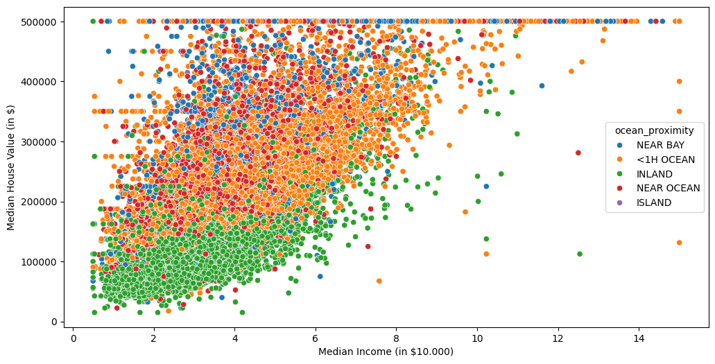
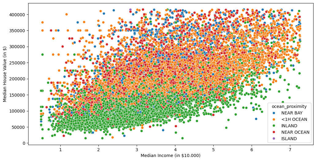
fig, ax = plt.subplots(figsize=(12,6))
sns.scatterplot(data=df, x='median_income', y='median_house_value', hue='ocean_proximity', ax=ax)
ax.set_ylabel('Median House Value (in $)')
ax.set_xlabel('Median Income (in $10.000)')

Text(0.5, 0, 'Median Income (in $10.000)')

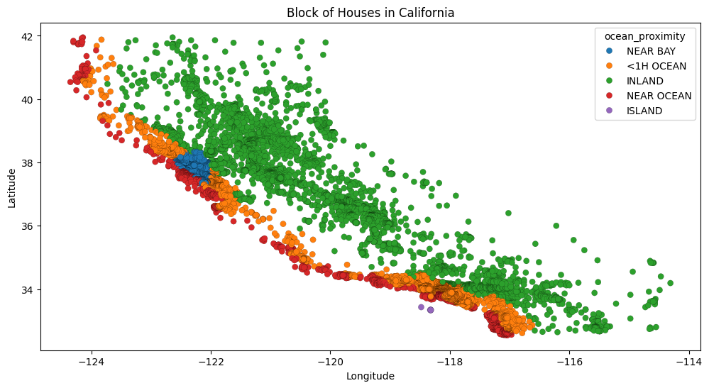
fig, ax = plt.subplots(figsize=(12,6))
sns.scatterplot(data=df, x='longitude', y='latitude', hue='ocean_proximity', edgecolor='black', linewidth=0.1)

ax.set_xlabel('Longitude')
ax.set_ylabel('Latitude')
ax.set_title('Block of Houses in California')

Text(0.5, 1.0, 'Block of Houses in California')

df_OceanProximityAgg = df.groupby(by='ocean_proximity').agg(
    {'median_income' : 'sum', 'median_house_value' : 'sum'}
    )
df_OceanProximityAgg = df_OceanProximityAgg.sort_values(by='median_house_value', ascending=False)

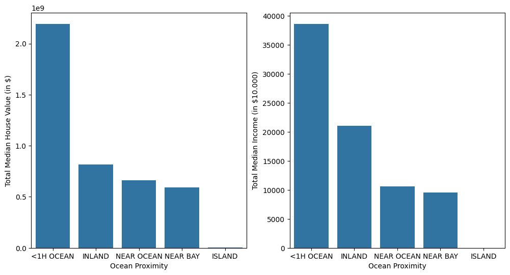
fig, ax = plt.subplots(figsize=(12,6), ncols=2)
sns.barplot(data=df_OceanProximityAgg, x='ocean_proximity', y='median_house_value', ax=ax[0])
ax[0].set_ylabel('Total Median House Value (in $)')
ax[0].set_xlabel('Ocean Proximity')

sns.barplot(data=df_OceanProximityAgg, x='ocean_proximity', y='median_income', ax=ax[1])
ax[1].set_ylabel('Total Median Income (in $10.000)')
ax[1].set_xlabel('Ocean Proximity')

Text(0.5, 0, 'Ocean Proximity')

For the ocean_proximity, it must be encoded to numerical data.

mapper = {'<1H OCEAN' : 1, 'INLAND' : 2, 'NEAR OCEAN' : 3, 'NEAR BAY' : 4, 'ISLAND' : 5}

df['ocean_proximity_encoded'] = df['ocean_proximity'].map(mapper)

df.head()

	longitude	latitude	housing_median_age	total_rooms	total_bedrooms	population	households	median_income	median_house_value	ocean_proximity	ocean_proximity_encoded
0	-122.23	37.88	41.0	880.0	129.0	322.0	126.0	8.3252	452600.0	NEAR BAY	4
1	-122.22	37.86	21.0	7099.0	1106.0	2401.0	1138.0	8.3014	358500.0	NEAR BAY	4
2	-122.24	37.85	52.0	1467.0	190.0	496.0	177.0	7.2574	352100.0	NEAR BAY	4
3	-122.25	37.85	52.0	1274.0	235.0	558.0	219.0	5.6431	341300.0	NEAR BAY	4
4	-122.25	37.85	52.0	1627.0	280.0	565.0	259.0	3.8462	342200.0	NEAR BAY	4

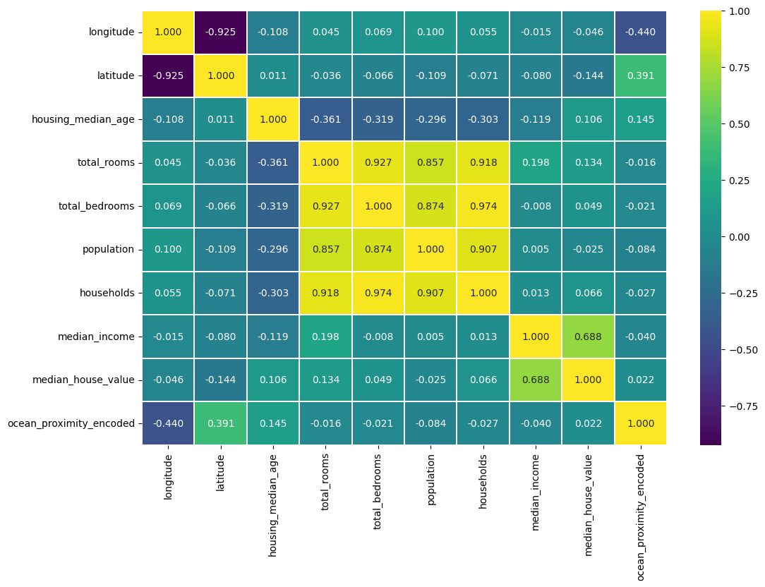
# plotting the pairplot to see the correlation for pair of features

fig, ax = plt.subplots(figsize=(12,8))
sns.heatmap(df.corr(numeric_only=True), cmap='viridis', linewidths=.2, fmt='.3f', annot=True, ax=ax)

<Axes: >

# Checking the outliers for numerical features
df_OnlyFloat = df.select_dtypes('float64')
df_OnlyFloatCols = df_OnlyFloat.columns

fig, ax = plt.subplots(figsize=(10,8), ncols=3, nrows=3)
k = 0
for i in range(3):
  for j in range(3):
    getFeatureCol = df_OnlyFloatCols[k]
    sns.boxplot(df_OnlyFloat[getFeatureCol], ax=ax[i][j])
    plt.tight_layout()
    k += 1

df_clean = df.copy(deep=True)

# Removing outlier using IQR method
features = ['total_rooms', 'total_bedrooms', 'population', 'households', 'median_income', 'median_house_value']
n_iteration = 6

for i in range(n_iteration):
  for feature in features:
    Q1 = df_clean[feature].quantile(0.25)
    Q3 = df_clean[feature].quantile(0.75)
    IQR = Q3 - Q1

    # Filtering
    lower_bound = Q1 - 1.5 * IQR
    upper_bound = Q3 + 1.5 * IQR
    df_clean = df_clean[(df_clean[feature] >= lower_bound) & (df_clean[feature] <= upper_bound)]

# Checking the outliers for numerical features
df_OnlyFloat = df_clean.select_dtypes('float64')
df_OnlyFloatCols = df_OnlyFloat.columns

fig, ax = plt.subplots(figsize=(10,8), ncols=3, nrows=3)
k = 0
for i in range(3):
  for j in range(3):
    getFeatureCol = df_OnlyFloatCols[k]
    sns.boxplot(df_OnlyFloat[getFeatureCol], ax=ax[i][j])
    plt.tight_layout()
    k += 1

# Checking the outliers for numerical features, except for longitude and latitude
df_OnlyFloat = df_clean.select_dtypes('float64')
df_OnlyFloatCols = df_OnlyFloat.columns

fig, ax = plt.subplots(figsize=(10,8), ncols=3, nrows=3)
k = 0
for i in range(3):
  for j in range(3):
    getFeatureCol = df_OnlyFloatCols[k]
    sns.histplot(df_OnlyFloat[getFeatureCol], kde=True, ax=ax[i][j])
    plt.tight_layout()
    k += 1

fig, ax = plt.subplots(figsize=(12,6))
sns.scatterplot(data=df_clean, x='median_income', y='median_house_value', hue='ocean_proximity', ax=ax)
ax.set_ylabel('Median House Value (in $)')
ax.set_xlabel('Median Income (in $10.000)')

Text(0.5, 0, 'Median Income (in $10.000)')

# plotting the pairplot to see the correlation for pair of features

fig, ax = plt.subplots(figsize=(12,8))
sns.heatmap(df_clean.corr(numeric_only=True), cmap='viridis', linewidths=.2, fmt='.3f', annot=True, ax=ax)

<Axes: >

# The median_income has clear positive correlation with the median house value
# The increasing the median income, the increase the median house value.
# However, the increasing median house value is less significant due to the total
# population, house median age, households, total rooms, and total bedrooms.
# In this case, the median_house_value is the target for creating a linear model
# The rest of features will be as the data

from sklearn.preprocessing import StandardScaler
from sklearn.linear_model import LinearRegression
from sklearn.metrics import r2_score, mean_squared_error, root_mean_squared_error, mean_absolute_percentage_error
from sklearn.model_selection import train_test_split

scaler = StandardScaler().set_output(transform="pandas")

y = df_clean['median_house_value']
x = df_clean.drop(['median_house_value', 'ocean_proximity', 'longitude', 'latitude'], axis=1)

# split the dataset into training and testing datasets
x_train, x_test, y_train, y_test = train_test_split(x, y, test_size=0.2, random_state=42)

# Scalling
x_train_scaled = scaler.fit_transform(x_train)
x_test_scaled = scaler.transform(x_test)

# Training the dataset using LinearRegression
linear_model = LinearRegression()
linear_model.fit(x_train_scaled, y_train)


y_pred = linear_model.predict(x_test_scaled)

# evaluating model
r2 = r2_score(y_test, y_pred)
rmse = root_mean_squared_error(y_test, y_pred)
mae_p = mean_absolute_percentage_error(y_test, y_pred)

print(f"R2: {r2:.4f}")
print(f"RMSE: {rmse:.4f}")
print(f"MAE(%): {mae_p:.4f}")

R2: 0.5113
RMSE: 59195.7423
MAE(%): 0.3103