Loan Eligibility Analysis#
Tentang Dataset#
Dataset berikut digunakan untuk memprediksi apakah calon peminjam memenuhi syarat untuk disetujui peminjamannya berdasarkan wilayah, keuangan, dan faktor yang berhubungan dengan kredit lainnta. Dataset ini cocok untuk klasifikasi menggunakan machine learning.
Dataset diperoleh dari repository Kaggle pada link berikut
https://www.kaggle.com/datasets/avineshprabhakaran/loan-eligibility-prediction
Dataset memiliki cakupan data sebagai berikut
Column |
Description |
Example |
|---|---|---|
Customer_ID |
Unique identifier for each loan applicant |
569 |
Gender |
Gender of the applicant |
Male / Female |
Married |
Marital status of the applicant |
Yes / No |
Dependents |
Number of dependents |
0, 1, 2, 3 |
Education |
Education level of the applicant |
Graduate / Not Graduate |
Self_Employed |
Whether the applicant is self-employed |
Yes / No |
Applicant_Income |
Applicant’s monthly income |
5000 |
Coapplicant_Income |
Coapplicant’s monthly income |
1500 |
Loan_Amount |
Loan amount requested (in thousands) |
128 |
Loan_Amount_Term |
Loan repayment term (in months) |
360 |
Credit_History |
Credit history meets lending criteria |
(1 = Yes, 0 = No) 1 |
Property_Area |
Type of property area |
Urban / Semiurban / Rural |
Loan_Status |
Loan approved or not (target variable) |
Y / N |
Import the library#
[1]:
import kagglehub
import os

import pandas as pd
import matplotlib.pyplot as plt
from matplotlib.ticker import MultipleLocator
import matplotlib as mpl
import seaborn as sns
Unduh Dataset#
[2]:
path = kagglehub.dataset_download("avineshprabhakaran/loan-eligibility-prediction")
filename = os.listdir(path)[0]

fullpath = "/".join([path,filename])
fullpath
Downloading to /root/.cache/kagglehub/datasets/avineshprabhakaran/loan-eligibility-prediction/3.archive...
100%|██████████| 7.39k/7.39k [00:00<00:00, 13.1MB/s]
Extracting files...
[2]:
'/root/.cache/kagglehub/datasets/avineshprabhakaran/loan-eligibility-prediction/versions/3/Loan Eligibility Prediction.csv'
Set the default plot style#
[3]:
def DefaultPlotStyle():
  plt.rcParams['lines.linewidth'] = 2
  plt.rcParams['lines.linestyle'] = '-'
  plt.rcParams['figure.figsize'] = [12,10]
  plt.rcParams['font.size'] = 12

DefaultPlotStyle()
Membaca Dataset#
[4]:
df = pd.read_csv(fullpath)
df.info()
<class 'pandas.core.frame.DataFrame'>
RangeIndex: 614 entries, 0 to 613
Data columns (total 13 columns):
 #   Column              Non-Null Count  Dtype
---  ------              --------------  -----
 0   Customer_ID         614 non-null    int64
 1   Gender              614 non-null    object
 2   Married             614 non-null    object
 3   Dependents          614 non-null    int64
 4   Education           614 non-null    object
 5   Self_Employed       614 non-null    object
 6   Applicant_Income    614 non-null    int64
 7   Coapplicant_Income  614 non-null    float64
 8   Loan_Amount         614 non-null    int64
 9   Loan_Amount_Term    614 non-null    int64
 10  Credit_History      614 non-null    int64
 11  Property_Area       614 non-null    object
 12  Loan_Status         614 non-null    object
dtypes: float64(1), int64(6), object(6)
memory usage: 62.5+ KB
Pengecekan Dataset#
[5]:
# Checking missing value
df.isnull().sum().reset_index().T
[5]:
| 0 | 1 | 2 | 3 | 4 | 5 | 6 | 7 | 8 | 9 | 10 | 11 | 12 | |
|---|---|---|---|---|---|---|---|---|---|---|---|---|---|
| index | Customer_ID | Gender | Married | Dependents | Education | Self_Employed | Applicant_Income | Coapplicant_Income | Loan_Amount | Loan_Amount_Term | Credit_History | Property_Area | Loan_Status |
| 0 | 0 | 0 | 0 | 0 | 0 | 0 | 0 | 0 | 0 | 0 | 0 | 0 | 0 |
Tidak ada data atau nilai yang kosong dalam dataset ini
[6]:
# Checking duplicate data
any(df.duplicated())
[6]:
False
[7]:
# Checking duplicate customer id
df['Customer_ID'].value_counts().reset_index().sort_values(by='count', ascending=False).head()
[7]:
| Customer_ID | count | |
|---|---|---|
| 613 | 271 | 1 |
| 0 | 606 | 1 |
| 1 | 569 | 1 |
| 2 | 15 | 1 |
| 3 | 95 | 1 |
Tidak ada data yang duplikat dalam dataset ini
Tampilan Dataset#
[8]:
df.head()
[8]:
| Customer_ID | Gender | Married | Dependents | Education | Self_Employed | Applicant_Income | Coapplicant_Income | Loan_Amount | Loan_Amount_Term | Credit_History | Property_Area | Loan_Status | |
|---|---|---|---|---|---|---|---|---|---|---|---|---|---|
| 0 | 569 | Female | No | 0 | Graduate | No | 2378 | 0.0 | 9 | 360 | 1 | Urban | N |
| 1 | 15 | Male | Yes | 2 | Graduate | No | 1299 | 1086.0 | 17 | 120 | 1 | Urban | Y |
| 2 | 95 | Male | No | 0 | Not Graduate | No | 3620 | 0.0 | 25 | 120 | 1 | Semiurban | Y |
| 3 | 134 | Male | Yes | 0 | Graduate | Yes | 3459 | 0.0 | 25 | 120 | 1 | Semiurban | Y |
| 4 | 556 | Male | Yes | 1 | Graduate | No | 5468 | 1032.0 | 26 | 360 | 1 | Semiurban | Y |
Analisis Parameter#
[9]:
# Creating object feature for Credit History
mapper = lambda x : "YES" if x == 1 else "NO"
df['Credit_History_Obj'] = df['Credit_History'].map(mapper)
df.head()
[9]:
| Customer_ID | Gender | Married | Dependents | Education | Self_Employed | Applicant_Income | Coapplicant_Income | Loan_Amount | Loan_Amount_Term | Credit_History | Property_Area | Loan_Status | Credit_History_Obj | |
|---|---|---|---|---|---|---|---|---|---|---|---|---|---|---|
| 0 | 569 | Female | No | 0 | Graduate | No | 2378 | 0.0 | 9 | 360 | 1 | Urban | N | YES |
| 1 | 15 | Male | Yes | 2 | Graduate | No | 1299 | 1086.0 | 17 | 120 | 1 | Urban | Y | YES |
| 2 | 95 | Male | No | 0 | Not Graduate | No | 3620 | 0.0 | 25 | 120 | 1 | Semiurban | Y | YES |
| 3 | 134 | Male | Yes | 0 | Graduate | Yes | 3459 | 0.0 | 25 | 120 | 1 | Semiurban | Y | YES |
| 4 | 556 | Male | Yes | 1 | Graduate | No | 5468 | 1032.0 | 26 | 360 | 1 | Semiurban | Y | YES |
[10]:
# Selecting only object features
object_list = df.select_dtypes(include=['object']).columns
object_list
[10]:
Index(['Gender', 'Married', 'Education', 'Self_Employed', 'Property_Area',
       'Loan_Status', 'Credit_History_Obj'],
      dtype='object')
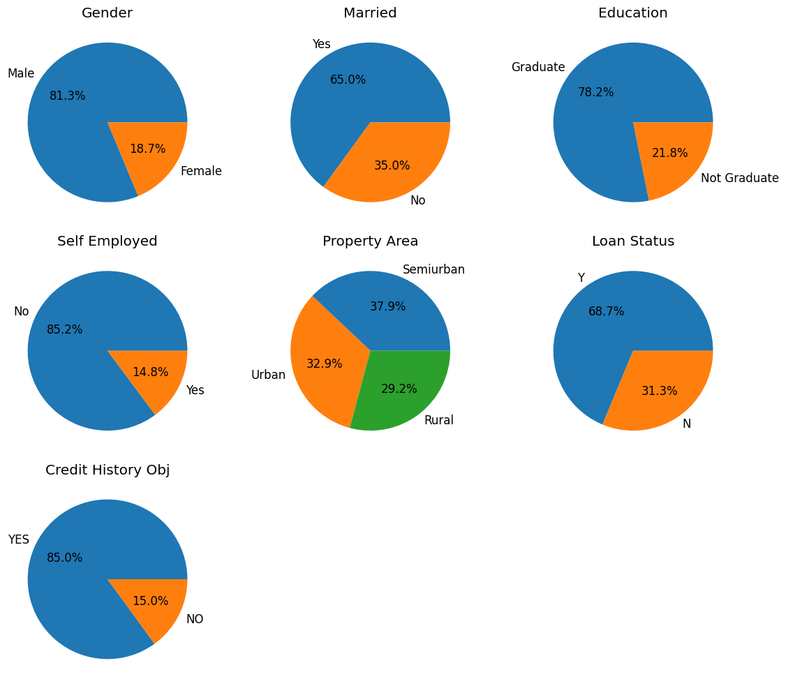
[11]:
# Plotting object features
ndata = df.shape[0]
nobject = len(object_list)
n_cols = 3
n_rows = (nobject // n_cols) + 1

fig, ax = plt.subplots(nrows=n_rows, ncols=n_cols)
ax_flat = ax.flatten()

for i, ax in enumerate(ax_flat):
  if i < nobject:
    df_obj = df[object_list[i]].value_counts().reset_index()
    df_obj['percentage'] = (df_obj['count']/df_obj['count'].sum()) * 100
    ax = ax_flat[i]
    ax.pie(df_obj['percentage'], labels=df_obj[object_list[i]], autopct="%.1f%%")
    ax.set_title(object_list[i].replace("_", " "))
  else:
    ax.axis('off')

plt.tight_layout()
[12]:
# Calculating the total income from the applicant income and co-applicant income
df['Total_Income'] = df['Applicant_Income'] + df['Coapplicant_Income']
df.head()
[12]:
| Customer_ID | Gender | Married | Dependents | Education | Self_Employed | Applicant_Income | Coapplicant_Income | Loan_Amount | Loan_Amount_Term | Credit_History | Property_Area | Loan_Status | Credit_History_Obj | Total_Income | |
|---|---|---|---|---|---|---|---|---|---|---|---|---|---|---|---|
| 0 | 569 | Female | No | 0 | Graduate | No | 2378 | 0.0 | 9 | 360 | 1 | Urban | N | YES | 2378.0 |
| 1 | 15 | Male | Yes | 2 | Graduate | No | 1299 | 1086.0 | 17 | 120 | 1 | Urban | Y | YES | 2385.0 |
| 2 | 95 | Male | No | 0 | Not Graduate | No | 3620 | 0.0 | 25 | 120 | 1 | Semiurban | Y | YES | 3620.0 |
| 3 | 134 | Male | Yes | 0 | Graduate | Yes | 3459 | 0.0 | 25 | 120 | 1 | Semiurban | Y | YES | 3459.0 |
| 4 | 556 | Male | Yes | 1 | Graduate | No | 5468 | 1032.0 | 26 | 360 | 1 | Semiurban | Y | YES | 6500.0 |
[13]:
fig, ax = plt.subplots(figsize=(12,6))
sns.countplot(data=df, x='Gender', hue='Loan_Status', ax=ax)
for container in ax.containers:
  ax.bar_label(container, label_type='edge')
# ax.set_ylim([0,200])
ax.set_ylabel('Number of Applicants')
ax.yaxis.set_minor_locator(MultipleLocator(25))
plt.grid(which='both')
plt.legend(title='Loan Status')
ax.set_axisbelow(True)
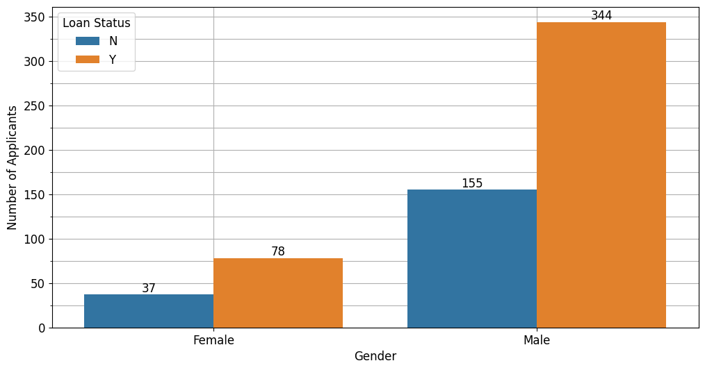
Berdasarkan jenis kelamin, peminjaman yang berhasil dilakukan secara mayoritas oleh pelanggan laki-kali, hanya kurang dari 100 pelanggan wanita yang berhasil mendapatkan pinjaman.
[14]:
fig, ax = plt.subplots(figsize=(12,6))
sns.countplot(data=df, x='Education',hue='Loan_Status', ax=ax)
for container in ax.containers:
  ax.bar_label(container, label_type='edge')
# ax.set_ylim([0,200])
ax.set_ylabel('Number of Applicants')
ax.yaxis.set_minor_locator(MultipleLocator(25))
plt.grid(which='both')
plt.legend(title='Loan Status')
ax.set_axisbelow(True)
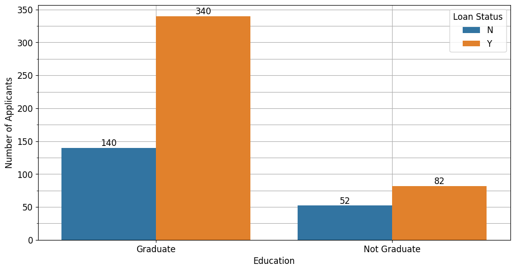
Berdasarkan status pendidikan, pelanggan yang lulus kuliah lebih berpeluang menerima pinjaman dibandingkan dengan pelanggan yang tidak lulus kuliah.
[15]:
fig, ax = plt.subplots(figsize=(12,6))
sns.countplot(data=df, x='Self_Employed', hue='Loan_Status', ax=ax)
for container in ax.containers:
  ax.bar_label(container, label_type='edge')
# ax.set_ylim([0,200])
ax.set_ylabel('Number of Applicants')
ax.yaxis.set_minor_locator(MultipleLocator(25))
plt.grid(which='both')
plt.legend(title='Loan Status')
ax.set_axisbelow(True)
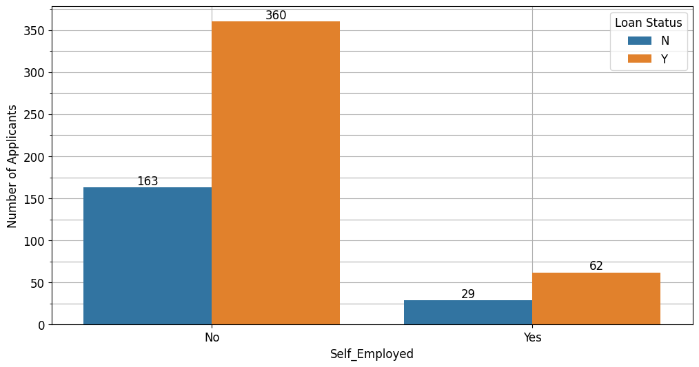
Berdasarkan status pekerjaan, pelanggan dengan status bukan wiraswasta berpeluang mendapatkan pinjaman.
[16]:
fig, ax = plt.subplots(figsize=(12,6))
sns.countplot(data=df, x='Property_Area', hue='Loan_Status', ax=ax)
for container in ax.containers:
  ax.bar_label(container, label_type='edge')
# ax.set_ylim([0,200])
ax.set_ylabel('Number of Applicants')
ax.yaxis.set_minor_locator(MultipleLocator(25))
plt.grid(which='both')
ax.set_axisbelow(True)
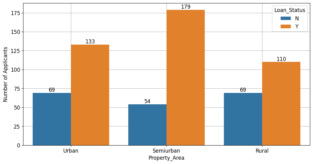
Berdasarkan wilayah tempat tinggal, peminjaman banyak diajukan oleh pelanggan yang tinggal di wilayah semiurban, diikuti dengan pelanggan yang tinggal di wilayah urban dan pedesaan.
[17]:
fig, ax = plt.subplots(figsize=(12,6))
sns.countplot(data=df, x='Dependents', hue='Loan_Status', ax=ax)
for container in ax.containers:
  ax.bar_label(container, label_type='edge')
# ax.set_ylim([0,200])
ax.set_ylabel('Number of Applicants')
ax.yaxis.set_minor_locator(MultipleLocator(25))
plt.grid(which='both')
ax.set_axisbelow(True)
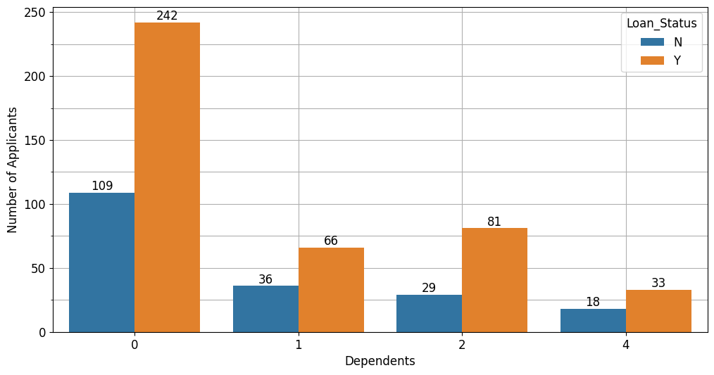
Mayoritas peminjaman yang diajukan dan diterima berasal dari pelanggan yang tidak memiliki tanggungan.
[18]:
fig, ax = plt.subplots(figsize=(12,6))
sns.countplot(data=df, x='Married', hue='Loan_Status', ax=ax)
for container in ax.containers:
  ax.bar_label(container, label_type='edge')
# ax.set_ylim([0,200])
ax.set_ylabel('Number of Applicants')
ax.yaxis.set_minor_locator(MultipleLocator(25))
plt.grid(which='both')
ax.set_axisbelow(True)
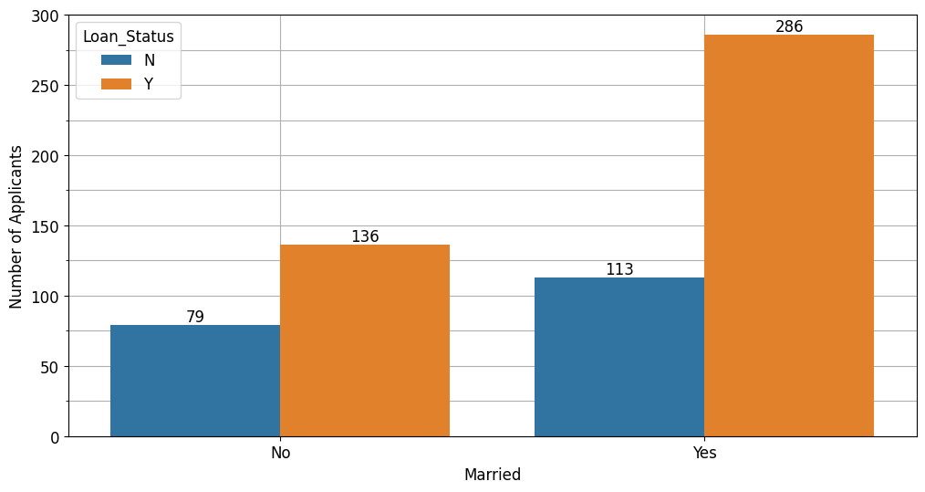
Berdasarkan status pernikahan, pelanggan dengan status sudah menikah berpeluang menerima pinjaman.
[20]:
fig, ax = plt.subplots(figsize=(12,6))
sns.countplot(data=df, x='Credit_History_Obj', hue='Loan_Status', ax=ax)
for container in ax.containers:
  ax.bar_label(container, label_type='edge')
# ax.set_ylim([0,200])
ax.set_ylabel('Number of Applicants')
ax.yaxis.set_minor_locator(MultipleLocator(25))
plt.grid(which='both')
ax.set_axisbelow(True)
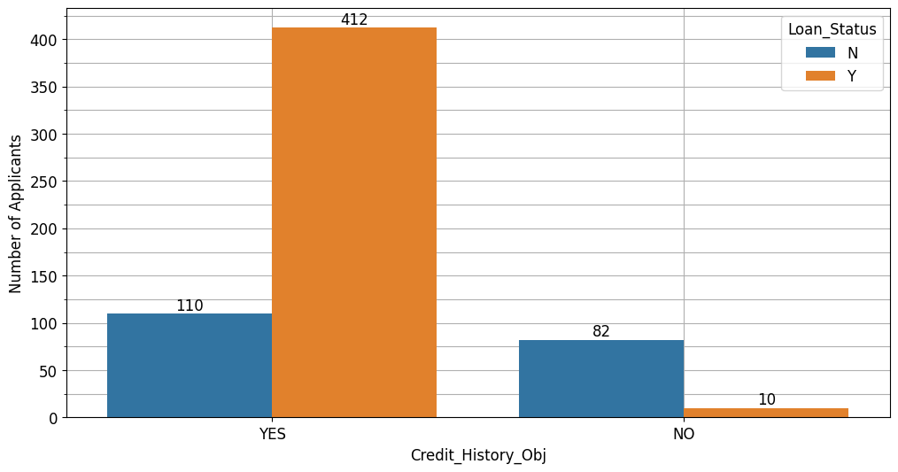
Berdasarkan rekam jejak peminjaman, pelanggan yang pernah melakukan peminjaman berpeluang mendapatkan pinjaman kembali.
[21]:
# Selecting only numeric data
numeric_list = df.select_dtypes(exclude=['object']).columns
numeric_list = numeric_list.delete(0)
numeric_list
[21]:
Index(['Dependents', 'Applicant_Income', 'Coapplicant_Income', 'Loan_Amount',
       'Loan_Amount_Term', 'Credit_History', 'Total_Income'],
      dtype='object')
[22]:
df_numeric = df.select_dtypes(exclude=['object'])
df_numeric.head()
[22]:
| Customer_ID | Dependents | Applicant_Income | Coapplicant_Income | Loan_Amount | Loan_Amount_Term | Credit_History | Total_Income | |
|---|---|---|---|---|---|---|---|---|
| 0 | 569 | 0 | 2378 | 0.0 | 9 | 360 | 1 | 2378.0 |
| 1 | 15 | 2 | 1299 | 1086.0 | 17 | 120 | 1 | 2385.0 |
| 2 | 95 | 0 | 3620 | 0.0 | 25 | 120 | 1 | 3620.0 |
| 3 | 134 | 0 | 3459 | 0.0 | 25 | 120 | 1 | 3459.0 |
| 4 | 556 | 1 | 5468 | 1032.0 | 26 | 360 | 1 | 6500.0 |
[23]:
df_numeric.drop('Customer_ID', axis=1, inplace=True)
df_numeric.head()
[23]:
| Dependents | Applicant_Income | Coapplicant_Income | Loan_Amount | Loan_Amount_Term | Credit_History | Total_Income | |
|---|---|---|---|---|---|---|---|
| 0 | 0 | 2378 | 0.0 | 9 | 360 | 1 | 2378.0 |
| 1 | 2 | 1299 | 1086.0 | 17 | 120 | 1 | 2385.0 |
| 2 | 0 | 3620 | 0.0 | 25 | 120 | 1 | 3620.0 |
| 3 | 0 | 3459 | 0.0 | 25 | 120 | 1 | 3459.0 |
| 4 | 1 | 5468 | 1032.0 | 26 | 360 | 1 | 6500.0 |
[24]:
df.describe()
[24]:
| Customer_ID | Dependents | Applicant_Income | Coapplicant_Income | Loan_Amount | Loan_Amount_Term | Credit_History | Total_Income | |
|---|---|---|---|---|---|---|---|---|
| count | 614.000000 | 614.000000 | 614.000000 | 614.000000 | 614.000000 | 614.000000 | 614.000000 | 614.000000 |
| mean | 307.500000 | 0.856678 | 5403.459283 | 1621.245798 | 142.022801 | 338.892508 | 0.850163 | 7024.705081 |
| std | 177.390811 | 1.216651 | 6109.041673 | 2926.248369 | 87.083089 | 69.716355 | 0.357203 | 6458.663872 |
| min | 1.000000 | 0.000000 | 150.000000 | 0.000000 | 9.000000 | 12.000000 | 0.000000 | 1442.000000 |
| 25% | 154.250000 | 0.000000 | 2877.500000 | 0.000000 | 98.000000 | 360.000000 | 1.000000 | 4166.000000 |
| 50% | 307.500000 | 0.000000 | 3812.500000 | 1188.500000 | 125.000000 | 360.000000 | 1.000000 | 5416.500000 |
| 75% | 460.750000 | 2.000000 | 5795.000000 | 2297.250000 | 164.750000 | 360.000000 | 1.000000 | 7521.750000 |
| max | 614.000000 | 4.000000 | 81000.000000 | 41667.000000 | 700.000000 | 480.000000 | 1.000000 | 81000.000000 |
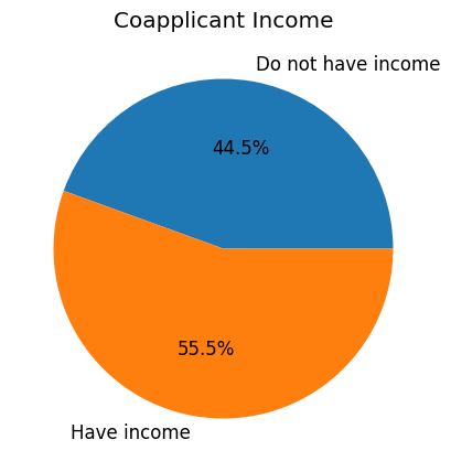
[25]:
number_Coapplicant_Income_zero = df[df['Coapplicant_Income'] == 0].shape[0]
number_Coapplicant_Income_nonzero = df.shape[0] - number_Coapplicant_Income_zero

percentage_Coapplicant_Income_zero = (number_Coapplicant_Income_zero/df.shape[0])*100
percentage_Coapplicant_Income_nonzero = (number_Coapplicant_Income_nonzero/df.shape[0])*100

fig, ax = plt.subplots(figsize=(5,5))
ax.pie(x= [percentage_Coapplicant_Income_zero, percentage_Coapplicant_Income_nonzero],
       labels=['Do not have income', 'Have income'],
       autopct="%.1f%%");
ax.set_title('Coapplicant Income')
[25]:
Text(0.5, 1.0, 'Coapplicant Income')
[26]:
# Encoding the object data to numeric
df_object = df.select_dtypes(include=['object'])
df_object.head()
[26]:
| Gender | Married | Education | Self_Employed | Property_Area | Loan_Status | Credit_History_Obj | |
|---|---|---|---|---|---|---|---|
| 0 | Female | No | Graduate | No | Urban | N | YES |
| 1 | Male | Yes | Graduate | No | Urban | Y | YES |
| 2 | Male | No | Not Graduate | No | Semiurban | Y | YES |
| 3 | Male | Yes | Graduate | Yes | Semiurban | Y | YES |
| 4 | Male | Yes | Graduate | No | Semiurban | Y | YES |
[27]:
gender_encoder = lambda x : 1 if x == 'Male' else 0
married_encoder = lambda x : 1 if x == 'Yes' else 0
education_encoder = lambda x : 1 if x == 'Graduate' else 0
self_employed_encoder = lambda x : 1 if x == 'Yes' else 0
property_area_encoder = lambda x : 1 if x == 'Urban' else 2 if x == 'Semiurban' else 3
loan_status_encoder = lambda x : 1 if x == 'Y' else 0

mappers = [gender_encoder, married_encoder, education_encoder, self_employed_encoder, property_area_encoder, loan_status_encoder]

df_object_names = df_object.columns.to_list()
df_object_names.remove('Credit_History_Obj')
df_object_names
[27]:
['Gender',
 'Married',
 'Education',
 'Self_Employed',
 'Property_Area',
 'Loan_Status']
[28]:
df_duplicate = df.copy(deep=True)

for i, obj in enumerate(df_object_names):
  df_duplicate[obj] = df_duplicate[obj].map(mappers[i])

df_duplicate.drop(['Customer_ID','Credit_History_Obj'], axis=1, inplace=True)
[29]:
df_duplicate.head()
[29]:
| Gender | Married | Dependents | Education | Self_Employed | Applicant_Income | Coapplicant_Income | Loan_Amount | Loan_Amount_Term | Credit_History | Property_Area | Loan_Status | Total_Income | |
|---|---|---|---|---|---|---|---|---|---|---|---|---|---|
| 0 | 0 | 0 | 0 | 1 | 0 | 2378 | 0.0 | 9 | 360 | 1 | 1 | 0 | 2378.0 |
| 1 | 1 | 1 | 2 | 1 | 0 | 1299 | 1086.0 | 17 | 120 | 1 | 1 | 1 | 2385.0 |
| 2 | 1 | 0 | 0 | 0 | 0 | 3620 | 0.0 | 25 | 120 | 1 | 2 | 1 | 3620.0 |
| 3 | 1 | 1 | 0 | 1 | 1 | 3459 | 0.0 | 25 | 120 | 1 | 2 | 1 | 3459.0 |
| 4 | 1 | 1 | 1 | 1 | 0 | 5468 | 1032.0 | 26 | 360 | 1 | 2 | 1 | 6500.0 |
Applying Logistic Regression#
[30]:
from sklearn.linear_model import LogisticRegression
from sklearn.model_selection import train_test_split
from sklearn.metrics import confusion_matrix, accuracy_score, classification_report, roc_curve, roc_auc_score
from sklearn.preprocessing import StandardScaler
import numpy as np
[31]:
target = df_duplicate['Loan_Status']
features = df_duplicate.drop('Loan_Status', axis=1)

# Splitting the dataset, the test dataset is 20% of the total dataset
X_train, X_test, y_train, y_test = train_test_split(features, target, test_size=0.2, random_state=42)

# Applying the standar scaler for the scaling unbalance scale of dataset
scaler = StandardScaler()
X_train_scaled = scaler.fit_transform(X_train)
X_test_scaled = scaler.transform(X_test)

# Applying the logistic regression
linreg_model = LogisticRegression()
linreg_model.fit(X_train_scaled,y_train)

# Predicting the test dataset (scaled)
y_pred = linreg_model.predict(X_test_scaled)

# Evaluating the accuracy of the model
print(f"Accuracy: {accuracy_score(y_pred, y_test)}")
Accuracy: 0.8211382113821138
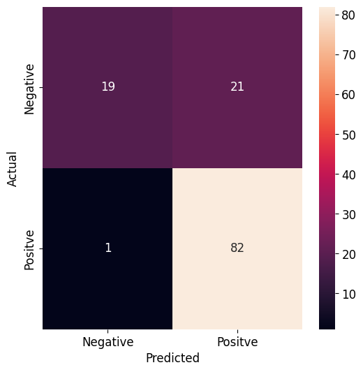
[32]:
# Providing the confusion matrix

# true negatives is C_{0,0},
# false positives is C_{0,1},
# false negatives is C_{1,0},
# true positives is C_{1,1}

custom_x_labels = ['Negative', 'Positve']
custom_y_labels = ['Negative', 'Positve']

fig, ax = plt.subplots(figsize=(6,6))
sns.heatmap(confusion_matrix(y_test, y_pred),
            xticklabels=custom_x_labels,
            yticklabels=custom_y_labels,
            annot=True,
            ax=ax)
ax.set_xlabel('Predicted')
ax.set_ylabel('Actual')
[32]:
Text(41.722222222222214, 0.5, 'Actual')
[33]:
# Generating the classification report
print(classification_report(y_pred, y_test, target_names=['Loan Status-No', 'Loan Status-Yes']));
                 precision    recall  f1-score   support

 Loan Status-No       0.47      0.95      0.63        20
Loan Status-Yes       0.99      0.80      0.88       103

       accuracy                           0.82       123
      macro avg       0.73      0.87      0.76       123
   weighted avg       0.90      0.82      0.84       123
Akurasi model sekitar 82% untuk memprediksi target (status peminjaman). Model ini cocok untuk memprediksi target sebenarnya (status pinjaman yang dapat diterima) sensitivitas (recall) 80%, tetapi lebih sensitif untuk memprediksi target status pinjaman yang tidak dapat diterima. Namun, model ini mampu memprediksi status pinjaman yang dapat diterima dengan presisi 99%.
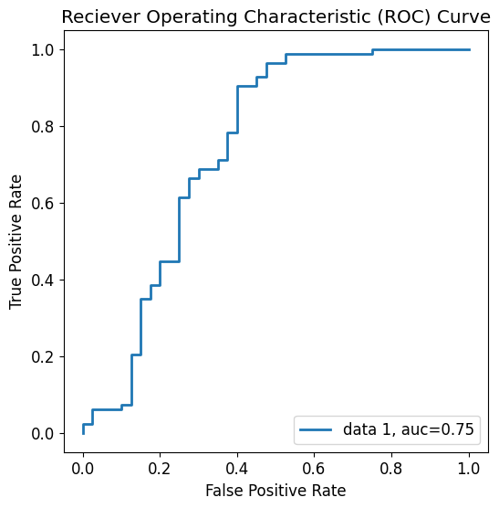
[34]:
# Plotting the ROC curve
y_pred_proba = linreg_model.predict_proba(X_test_scaled)[::,1]
fpr, tpr, _ = roc_curve(y_test,  y_pred_proba)
auc = roc_auc_score(y_test, y_pred_proba)

fig, ax = plt.subplots(figsize=(6,6))
ax.plot(fpr,tpr,label=f"data 1, auc={auc:.2f}")
ax.set_xlabel('False Positive Rate')
ax.set_ylabel('True Positive Rate')
ax.set_title('Reciever Operating Characteristic (ROC) Curve')
plt.legend(loc=4)
plt.show()