Seismic Hazard Curve: The Probability of Exceedance#

Aulia Khalqillah, S.Si., M.Si.

Tsunami and Disaster Mitigation Research Center (TDMRC)

Universitas Syiah Kuala, Banda Aceh, Indonesia

auliakhalqillah@usk.ac.id,

What is Seismic Hazard Curve?#

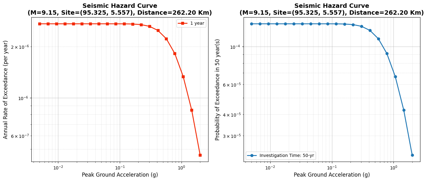
The seismic hazard curve describes the likelihood of an intensity measure type (IMT), such as PGA, PGV or PGD, that exceeds a certain IML, \(x\), given the probability of ground motion due to the magnitude ranges and distance ranges from a rupture source corresponding to a annual rate of exceedance. Mathematically, the annual rate of exceedance (\(\lambda [IMT \ge x]\)) can be calculated using the following formula

\(\lambda [IMT \ge x] = \Sigma_{source_i}^{n_{source}} \lambda_i(M \ge M_{min}) \int_{M_0}^{M_{max}} \int_{R|M} P[IMT \ge x | M,R] f(M) f(R|M) dr dm\)

where

\(n_{source}\) is total number seismic sources (ruptures)
\(\lambda_i(M \ge M_{min})\) is an annual rate (or annual occurrrence rate) of rupture
\(P[IMT \ge x | M,R]\) is the conditional probability of ground motion given a magnitude and distance that an IMT exceed an IML, \(x\)
\(f(M)\) is the Probability Density Function (PDF) of a magnitude
\(f(R|M)\) is the Probability Density Function (PDF) of a distance given a magnitude

Using the annual rate of exceedance, we can calculate the probability of exceedance (PoE) using the Poissonian probability formula

\(P(IMT \ge x) = 1 - e^{-\lambda[IMT \ge x] t}\)

The probability of exceedance describes the likelihood (probability) of various intensity levels that exceed a certain level of \(x\) over a time range (e.g, 50-yr of building age). The easiest way to explain this is to answer the question of what is the probability of an intensity level that exceeds to a certain level \(x\)?

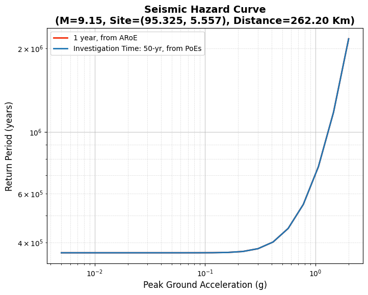
The annual rate of exceedance and probability of exceedance have relationship with return period as written in the equation below

\(RP = \frac {1}{\lambda [IMT \ge x]} = \frac {-t}{ln(1-P(IMT \ge x))}\)

The return period describes the average time for an event to occur at least once, given a specific magnitude (intensity) or greater, where \(t\) is the investigation time.

There are some steps to calculate the annual rate of exceedance and probability of exceedance as written below:

Calculating (or estimating) the occurrence rate of seismic sources (\(\lambda_i(M \ge M_{min})\))
Calculating the ground motion intensity using ground motion prediction equations (GMPEs)
Calculating the conditional probability of ground motion given magnitude and distance (\(P[IMT \ge x | M,R]\))
Calculating the probability density function (PDF) of magnitude (\(f(m)\))
Calculating the probability density function (PDF) of distance (\(f(R|M)\))
Calculating the annual rate of exceedance (\(\lambda [IMT \ge x]\))
Calculating the probability of exceedance given time range estimation (\(P(IMT \ge x)\))
Plotting the seismic hazard curve

Some Uncertainties to Produce Seismic Hazard Curve#

A seismic hazard curve will be generated at several grid points with a certain grid spacing covering a region of interest. Each point of the seismic hazard curve has its own IML and annual rate of exceedance or probability of exceedance that depends on the generated seismic source types. There are a number of seismic source types, namely Active Shallow Crust (ASC), Subduction Interface (SubInter), Subduction IntraSlab (SubIntra), and Background Source (BS). Each seismic source (rupture) has its own occurrence rate or annual rate of rupture (\(\lambda (M \ge M_{min})\)) based on its magnitude-frequency distribution. In subduction zones, its occurrence rate can be estimated by using the Magnitude-Frequency Distribution (MFD) of truncated Gutenberg-Richter’s Law (truncated GR), and for the active shallow crust can be estimated by using the MFD Youngs-Coppersmith Characteristics 1985 approach. These differences arise from the fact that the generated earthquake characteristics are different.

References#

Example Case#

I will demonsrate the probability of exceedance calculation and produce a seismic hazard curve at a certain site of interest. I will use a simple case of Aceh-Andaman Megathrust Segment (single rupture), Indonesia and a single magnitude of interest. The megathrust has a seismicity parameters of

a-value = 5.07
b-value = 0.91

Furthermore, the hazard will be estimated based on some parameters below

Minimum magnitude (Mw) = 7.0
Maximum magnitude (Mw) = 9.2
Bin of magnitude = 0.1
Magnitude of interest (Mw) = 9.15
Hypocenter depth (Km) = 13.5
Site characterization, Vs30 (m/s) = 760
Top-of-Rupture’s edged depth to the surface (Ztor) in Km = 3
Investigation time of exposure (year) = 50
Source Location (Lon, Lat) = 95.982, 3.295
Site Location (Lon, Lat) = 95.325, 5.557

where the main earthquake is based on the Mw 9.2 2004 Aceh, Sumatra Earthquake-Tsunami (see here from USGS’s report).

Note: This calculation is conducted using Python in Google Colab and OpenQuake Engine version 3.25.1 ***

[15]:

# Ignore this command if you execute the program from your local computer. Make sure that you have installed the latest OpenQuake engine
!pip install openquake.engine fiona

Requirement already satisfied: openquake.engine in /usr/local/lib/python3.12/dist-packages (3.25.1)
Requirement already satisfied: fiona in /usr/local/lib/python3.12/dist-packages (1.10.1)
Requirement already satisfied: setuptools in /usr/local/lib/python3.12/dist-packages (from openquake.engine) (75.2.0)
Requirement already satisfied: h5py>=2.10 in /usr/local/lib/python3.12/dist-packages (from openquake.engine) (3.16.0)
Requirement already satisfied: h3>=3.7 in /usr/local/lib/python3.12/dist-packages (from openquake.engine) (4.5.0)
Requirement already satisfied: numpy>=1.20 in /usr/local/lib/python3.12/dist-packages (from openquake.engine) (2.0.2)
Requirement already satisfied: numba>=0.58 in /usr/local/lib/python3.12/dist-packages (from openquake.engine) (0.60.0)
Requirement already satisfied: scipy>=1.3 in /usr/local/lib/python3.12/dist-packages (from openquake.engine) (1.16.3)
Requirement already satisfied: pandas>=0.25 in /usr/local/lib/python3.12/dist-packages (from openquake.engine) (2.2.2)
Requirement already satisfied: pyzmq>=19.0 in /usr/local/lib/python3.12/dist-packages (from openquake.engine) (26.2.1)
Requirement already satisfied: psutil>=2.0 in /usr/local/lib/python3.12/dist-packages (from openquake.engine) (5.9.5)
Requirement already satisfied: shapely>=1.7 in /usr/local/lib/python3.12/dist-packages (from openquake.engine) (2.1.2)
Requirement already satisfied: docutils>=0.11 in /usr/local/lib/python3.12/dist-packages (from openquake.engine) (0.21.2)
Requirement already satisfied: decorator>=4.3 in /usr/local/lib/python3.12/dist-packages (from openquake.engine) (4.4.2)
Requirement already satisfied: django<5,>=4.2 in /usr/local/lib/python3.12/dist-packages (from openquake.engine) (4.2.30)
Requirement already satisfied: matplotlib in /usr/local/lib/python3.12/dist-packages (from openquake.engine) (3.10.0)
Requirement already satisfied: requests>=2.20 in /usr/local/lib/python3.12/dist-packages (from openquake.engine) (2.32.4)
Requirement already satisfied: toml>=0.10.2 in /usr/local/lib/python3.12/dist-packages (from openquake.engine) (0.10.2)
Requirement already satisfied: pyproj>=1.9 in /usr/local/lib/python3.12/dist-packages (from openquake.engine) (3.7.2)
Requirement already satisfied: alpha_shapes>=1.1.0 in /usr/local/lib/python3.12/dist-packages (from openquake.engine) (1.1.1)
Requirement already satisfied: attrs>=19.2.0 in /usr/local/lib/python3.12/dist-packages (from fiona) (26.1.0)
Requirement already satisfied: certifi in /usr/local/lib/python3.12/dist-packages (from fiona) (2026.5.20)
Requirement already satisfied: click~=8.0 in /usr/local/lib/python3.12/dist-packages (from fiona) (8.4.1)
Requirement already satisfied: click-plugins>=1.0 in /usr/local/lib/python3.12/dist-packages (from fiona) (1.1.1.2)
Requirement already satisfied: cligj>=0.5 in /usr/local/lib/python3.12/dist-packages (from fiona) (0.7.2)
Requirement already satisfied: asgiref<4,>=3.6.0 in /usr/local/lib/python3.12/dist-packages (from django<5,>=4.2->openquake.engine) (3.11.1)
Requirement already satisfied: sqlparse>=0.3.1 in /usr/local/lib/python3.12/dist-packages (from django<5,>=4.2->openquake.engine) (0.5.5)
Requirement already satisfied: llvmlite<0.44,>=0.43.0dev0 in /usr/local/lib/python3.12/dist-packages (from numba>=0.58->openquake.engine) (0.43.0)
Requirement already satisfied: python-dateutil>=2.8.2 in /usr/local/lib/python3.12/dist-packages (from pandas>=0.25->openquake.engine) (2.9.0.post0)
Requirement already satisfied: pytz>=2020.1 in /usr/local/lib/python3.12/dist-packages (from pandas>=0.25->openquake.engine) (2025.2)
Requirement already satisfied: tzdata>=2022.7 in /usr/local/lib/python3.12/dist-packages (from pandas>=0.25->openquake.engine) (2026.2)
Requirement already satisfied: charset_normalizer<4,>=2 in /usr/local/lib/python3.12/dist-packages (from requests>=2.20->openquake.engine) (3.4.7)
Requirement already satisfied: idna<4,>=2.5 in /usr/local/lib/python3.12/dist-packages (from requests>=2.20->openquake.engine) (3.18)
Requirement already satisfied: urllib3<3,>=1.21.1 in /usr/local/lib/python3.12/dist-packages (from requests>=2.20->openquake.engine) (2.5.0)
Requirement already satisfied: contourpy>=1.0.1 in /usr/local/lib/python3.12/dist-packages (from matplotlib->openquake.engine) (1.3.3)
Requirement already satisfied: cycler>=0.10 in /usr/local/lib/python3.12/dist-packages (from matplotlib->openquake.engine) (0.12.1)
Requirement already satisfied: fonttools>=4.22.0 in /usr/local/lib/python3.12/dist-packages (from matplotlib->openquake.engine) (4.63.0)
Requirement already satisfied: kiwisolver>=1.3.1 in /usr/local/lib/python3.12/dist-packages (from matplotlib->openquake.engine) (1.5.0)
Requirement already satisfied: packaging>=20.0 in /usr/local/lib/python3.12/dist-packages (from matplotlib->openquake.engine) (26.2)
Requirement already satisfied: pillow>=8 in /usr/local/lib/python3.12/dist-packages (from matplotlib->openquake.engine) (11.3.0)
Requirement already satisfied: pyparsing>=2.3.1 in /usr/local/lib/python3.12/dist-packages (from matplotlib->openquake.engine) (3.3.2)
Requirement already satisfied: six>=1.5 in /usr/local/lib/python3.12/dist-packages (from python-dateutil>=2.8.2->pandas>=0.25->openquake.engine) (1.17.0)

[16]:

import numpy as np
from scipy.stats import norm
import matplotlib.pyplot as plt

from openquake.hazardlib.gsim.abrahamson_2014 import AbrahamsonEtAl2014
from openquake.hazardlib.gsim import get_available_gsims
from openquake.hazardlib.imt import PGA
from openquake.hazardlib.geo.geodetic import distance
from openquake.hazardlib.mfd.truncated_gr import TruncatedGRMFD
from openquake.hazardlib.valid import logscale

[17]:

gsims = get_available_gsims()
gmpe_list = ["ZhaoEtAl2006SInter"]

for name in gmpe_list:
    # 1. Instantiate the GMPE class object
    gmpe_instance = gsims[name]()

    print(f"=== Requirements for {name} ===")

    # 2. Site parameters required (e.g., vs30, backarc, z1pt0, etc)
    site_reqs = getattr(gmpe_instance, 'REQUIRES_SITES_PARAMETERS', set())
    print(f"Required Site Params   : {list(site_reqs)}")

    # 3. Rupture parameters required (e.g., mag, rake, dip, ztor)
    rup_reqs = getattr(gmpe_instance, 'REQUIRES_RUPTURE_PARAMETERS', set())
    print(f"Required Rupture Params: {list(rup_reqs)}")

    # 4. Metric distances required (e.g., rrup, rjb, rx)
    dist_reqs = getattr(gmpe_instance, 'REQUIRES_DISTANCES', set())
    print(f"Required Distances     : {list(dist_reqs)}")

    # 5. Tectonic Region details
    tr_type = gmpe_instance.DEFINED_FOR_TECTONIC_REGION_TYPE
    print(f"Tectonic Region Type   : {tr_type}\n")


# A. Data type definition
ctx_dtype = [
    ('mag', 'f8'),          # Magnitude
    ('rake', 'f8'),         # Rake angle
    ('dip', 'f8'),          # Dip angle
    ('ztor', 'f8'),         # Top depth of rupture
    ('width', 'f8'),        # Rupture width
    ('rrup', 'f8'),         # Rrup distance
    ('rjb', 'f8'),          # Rjb distance
    ('rx', 'f8'),           # Rx distance
    ('ry0', 'f8'),          # Ry0 distance
    ('vs30', 'f8'),         # Vs30 (local site)
    ('z1pt0', 'f8'),        # Depth of 1.0 Km/s
    ('z2pt5', 'f8'),        # Depth of 2.5 Km/s
    ('vs30measured', '?'),   # Boolean (?): True jika diukur, False jika estimasi
    ('backarc', '?')   # Boolean (?): True jika diukur, False jika estimasi
]

# 1. Calculating (or estimating) the occurrence rate of seismic sources
minMag, maxMag, binMag = 7.0, 9.2, 0.1
aval, bval = 5.07, 0.91
grMFD = TruncatedGRMFD(minMag, maxMag, binMag, aval, bval)
mag_rate_gr = grMFD.get_annual_occurrence_rates()

# Finding the closest value of magnitude
mag_of_interest = 9.15
closest_mag = min(mag_rate_gr, key=lambda m: abs(m[0] - mag_of_interest))
occurrence_rate = closest_mag[1]
print(f"Mag: {closest_mag[0]:.2f}\nOccurrence rate: {closest_mag[1]:.10f}\nRP_M: {int(1/closest_mag[1])}")

=== Requirements for ZhaoEtAl2006SInter ===
Required Site Params   : ['vs30']
Required Rupture Params: ['mag', 'hypo_depth']
Required Distances     : ['rrup']
Tectonic Region Type   : TRT.SUBDUCTION_INTERFACE

Mag: 9.15
Occurrence rate: 0.0001162924
RP_M: 8599

[18]:

# Source and target site definition
lon_source, lat_source, depth_source = 95.982, 3.295, 13.5
lon_site, lat_site, depth_site = 95.325, 5.557, 0

# Calculating the distance between source and target site
distance_value = distance(lon_source, lat_source, depth_source, lon_site, lat_site, depth_site)

[19]:

# B. Alocating the array of target size
num_sites = 1
ctx_array = np.zeros(num_sites, dtype=ctx_dtype)

# C. Formating the array to recarray
ctx = ctx_array.view(np.recarray)

# D. Defining some parameter values
ctx.mag = mag_of_interest
ctx.hypo_depth = 13.5
ctx.rake = 0.0
ctx.dip = 45.0
ctx.ztor = 3.0

ctx.repi = np.array([distance_value])
ctx.rhypo = np.sqrt(ctx.repi** 2.0 + ctx.hypo_depth**2.0)
ctx.rjb = ctx.repi
ctx.rrup = np.sqrt(ctx.rjb**2.0 + ctx.ztor**2)
ctx.rx = ctx.rjb

# ry0 adalah jarak horizontal terpendek dari lokasi stasiun/situs (site) ke garis batas
# samping patahan, diukur sejajar dengan arah jurus (strike) patahan. Nilai 0 asumsi sumbernya adalah titik
ctx.ry0 = np.array([0.0])

ctx.vs30 = np.array([760.0])
ctx.z1pt0 = np.array([41.30])
ctx.z2pt5 = np.array([0.6])
ctx.vs30measured = np.array([False])

[20]:

# Defining the intensity measure type
imts = [PGA()]

# Identification of dimension
shape = (len(imts), len(ctx))

# Alocating initial parameter for output (mean, sig, tau, and phi)
mean = np.zeros(shape, dtype='f8') # mean of ground motion value (in ln)
sig  = np.zeros(shape, dtype='f8') # Total Standard Deviation (sqrt(tau^2 + phi^2))
tau  = np.zeros(shape, dtype='f8') # Inter-event Standard Deviation
phi  = np.zeros(shape, dtype='f8') # Intra-event Standard Deviation

# Computing the intensity
gmpe_instance.compute(ctx, imts, mean, sig, tau, phi)
gmv = np.exp(mean[0])

# Calculating the total standard deviation
sig = np.sqrt(tau**2 + phi**2)
gmv_std = sig[0]

# Providing the result
print("HASIL PERHITUNGAN")
for i in range(num_sites):
    print(f"Lokasi {i+1} - Lon: {lon_site}, Lat: {lat_site} | Mean (ln) = {mean[0, i]:.5f} | PGA (g) = {np.exp(mean[0, i]):.5f} | Total Sigma = {sig[0, i]:.5f}")

HASIL PERHITUNGAN
Lokasi 1 - Lon: 95.325, Lat: 5.557 | Mean (ln) = -3.09519 | PGA (g) = 0.04527 | Total Sigma = 0.67800

[21]:

# 3. Calculating the conditional probability of ground motion given magnitude and distance ($P[IMT \ge x | M,R]$)
# Intensity Measure Levels (IMLs) for PGA in g\
imls = logscale(0.005, 2, 20)
prob_gmv = 1.0 - norm.cdf((np.log(imls) - gmv) / gmv_std)
prob_gmv

[21]:

array([1.        , 1.        , 1.        , 1.        , 1.        ,
       0.99999999, 0.99999982, 0.99999813, 0.99998413, 0.99989026,
       0.99938185, 0.99715617, 0.98928039, 0.9667511 , 0.91464838,
       0.81722547, 0.66993599, 0.48988024, 0.31189898, 0.16964213])

[22]:

# 4. Calculating the probability density function (PDF) of magnitude ($f(m)$)

def magPDF(mag, mag_max=None, mag_min=None, b_value = 1):
    '''
    The calculation of Probability Density Function (PDF) using truncated Gutenberg-Richter Law.

    See the equation B.17 in the OpenQuake Engine Testing Procedures

    Input

    :mag: Magnitude

    :mag_max: Maximum Magnitude

    :mag_min: Minimum Magnitude

    :b_value: The statistical parameter of seismicity. It can be determined using regression of GR-Law or Maximum Likelihood. Default is 1

    '''
    if mag_max == None or mag_min == None:
        mag_pdf = (b_value * np.log(10)*10**(-1 * b_value * mag))
    else:
        delta_mag = mag_max - mag_min
        mag_pdf = (b_value * np.log(10)*10**(-1 * b_value * (mag - mag_min))) / (1 - (10**(-1 * b_value * delta_mag)))

    return mag_pdf

# Calculating probability density function (PDF) for magnitude, assuming there is no minimum and maximum magnitude defined, also b-value is 1
MagPDF = magPDF(magnitude, maxMag, minMag, bval)
# MagPDF = 1
print(MagPDF)

0.023393851637878247

[23]:

# 5. Calculating the probability density function (PDF) of distance ($f(R|M)$)
# Assuming the probability density function for distance at site of interest is 1 based on dirac delta function
DistPDF = 1

[24]:

# 6. Calculating the annual rate of exceedance ($\lambda [IMT \ge x]$)
annual_rate_of_exceedance = occurrence_rate * prob_gmv * MagPDF * DistPDF
print(annual_rate_of_exceedance)

[2.72052681e-06 2.72052681e-06 2.72052681e-06 2.72052681e-06
 2.72052680e-06 2.72052677e-06 2.72052632e-06 2.72052173e-06
 2.72048363e-06 2.72022826e-06 2.71884511e-06 2.71279008e-06
 2.69136382e-06 2.63007229e-06 2.48832544e-06 2.22328379e-06
 1.82257883e-06 1.33273234e-06 8.48529525e-07 4.61515952e-07]

[25]:

# 7. Calculating the probability of exceedance given time range estimation ($P(IMT \ge x)$)
investigation_time = 50 # year
poes = 1 - np.exp(-1 * annual_rate_of_exceedance * investigation_time)
poes

[25]:

array([1.36017089e-04, 1.36017089e-04, 1.36017089e-04, 1.36017089e-04,
       1.36017089e-04, 1.36017087e-04, 1.36017065e-04, 1.36016835e-04,
       1.36014930e-04, 1.36002164e-04, 1.35933016e-04, 1.35630306e-04,
       1.34559137e-04, 1.31494968e-04, 1.24408533e-04, 1.11158011e-04,
       9.11247895e-05, 6.66343966e-05, 4.24255762e-05, 2.30755314e-05])

[26]:

fig, ax = plt.subplots(figsize=(16,6), ncols=2)

# Plot Annual Rate of Exceedance vs. IMLs on a log-log scale
ax[0].loglog(imls, annual_rate_of_exceedance, marker='s', linestyle='-', color="#f32a06", linewidth=2, markersize=6, label=f'1 year')

# Formatting the chart to look professional
ax[0].set_title(f'Seismic Hazard Curve\n(M={mag_of_interest}, Site={lon_site, lat_site}, Distance={ctx.repi[0]:.2f} Km)', fontsize=14, fontweight='bold')
ax[0].set_xlabel('Peak Ground Acceleration (g)', fontsize=12)
ax[0].set_ylabel('Annual Rate of Exceedance (per year)', fontsize=12)

# Adding grid lines for both major and minor ticks (crucial for log scales)
ax[0].grid(True, which="major", linestyle='-', linewidth=0.7, alpha=0.8)
ax[0].grid(True, which="minor", linestyle='--', linewidth=0.5, alpha=0.5)

ax[0].legend()

# Plot Annual Rate of Exceedance vs. IMLs on a log-log scale
ax[1].loglog(imls, poes, marker='o', linestyle='-', color='#1f77b4', linewidth=2, markersize=6, label=f'Investigation Time: {investigation_time}-yr')
# ax[0].loglog(imls, annual_rate_of_exceedance, marker='s', linestyle='--', color="#f32a06", linewidth=2, markersize=6, label='Annual Rate of Exceedance')

# Formatting the chart to look professional
ax[1].set_title(f'Seismic Hazard Curve\n(M={mag_of_interest}, Site={lon_site, lat_site}, Distance={ctx.repi[0]:.2f} Km)', fontsize=14, fontweight='bold')
ax[1].set_xlabel('Peak Ground Acceleration (g)', fontsize=12)
ax[1].set_ylabel(f'Probability of Exceedance in {investigation_time} year(s)', fontsize=12)

# Adding grid lines for both major and minor ticks (crucial for log scales)
ax[1].grid(True, which="major", linestyle='-', linewidth=0.7, alpha=0.8)
ax[1].grid(True, which="minor", linestyle='--', linewidth=0.5, alpha=0.5)

ax[1].legend()

[26]:

<matplotlib.legend.Legend at 0x79dd745aba40>

_images/Seismic_Hazard_Curve_OQ_13_1.png

[27]:

# Calculating return period from annual rate of exceedance
rp_are = 1/annual_rate_of_exceedance

# Calculating return period from probability of exceedance
rp_poes = (-1*investigation_time) / (np.log(1-poes))

[29]:

fig, ax = plt.subplots(figsize=(8,6), ncols=1)

# Plot Annual Rate of Exceedance vs. IMLs on a log-log scale
ax.loglog(imls, rp_are, marker='', linestyle='-', color="#f32a06", linewidth=2, markersize=6, label=f'1 year, from ARoE')
ax.loglog(imls, rp_poes, marker='', linestyle='-', color='#1f77b4', linewidth=2, markersize=6, label=f'Investigation Time: {investigation_time}-yr, from PoEs')

# Formatting the chart to look professional
ax.set_title(f'Seismic Hazard Curve\n(M={mag_of_interest}, Site={lon_site, lat_site}, Distance={ctx.repi[0]:.2f} Km)', fontsize=14, fontweight='bold')
ax.set_xlabel('Peak Ground Acceleration (g)', fontsize=12)
ax.set_ylabel('Return Period (years)', fontsize=12)

# Adding grid lines for both major and minor ticks (crucial for log scales)
ax.grid(True, which="major", linestyle='-', linewidth=0.7, alpha=0.8)
ax.grid(True, which="minor", linestyle='--', linewidth=0.5, alpha=0.5)

ax.legend()

[29]:

<matplotlib.legend.Legend at 0x79dd74a0dc40>

_images/Seismic_Hazard_Curve_OQ_15_1.png

[30]:

# get a certain annual rate of exceedance based on a specific IML
specificIML = 1 # in g
get_spec_annual_rate_of_exceedance = min(zip(imls, annual_rate_of_exceedance), key=lambda x: abs(x[0] - specificIML))

# get a certain probability of exceeance base on a specific IML
get_spec_poes = min(zip(imls, poes), key=lambda x: abs(x[0] - specificIML))
get_spec_poes

print(f"Annual Rate of Exceedance equal to or greater than {get_spec_annual_rate_of_exceedance[0]:.4f} g is {get_spec_annual_rate_of_exceedance[1]:.10f} with the probability of exceedance {get_spec_poes[1]*100:.10f} %")
print(f"Return Period for given or greater than {get_spec_annual_rate_of_exceedance[0]:.4f} g is {int(1/get_spec_annual_rate_of_exceedance[1])} years")
print(f"or equivalent to the PoEs {get_spec_poes[1]*100:.10f} % in {investigation_time} years")

Annual Rate of Exceedance equal to or greater than 1.0645 g is 0.0000013327 with the probability of exceedance 0.0066634397 %
Return Period for given or greater than 1.0645 g is 750338 years
or equivalent to the PoEs 0.0066634397 % in 50 years

Conclusion#

In this exercise, an \(M_w\) 9.15 earthquake from the Aceh-Andaman megathrust segment was simulated using a simple probabilistic seismic hazard calculation (with a single magnitude), yielding a seismic hazard curve as the final result. The distance from the earthquake source to the specific site is approximately 262.2 km. According to the Magnitude-Frequency Distribution (MFD) analysis using a truncated Gutenberg-Richter approach, this specific \(M_w\) 9.15 earthquake has an estimated annual occurrence rate of 0.000116 (equivalent to a return period of 8,599 years). Based on this magnitude occurrence rate, the site of interest is expected to experience an annual rate of exceedance of 0.0000013327 for a Peak Ground Acceleration (PGA) equal to or greater than 1.0645 g. This corresponds to a return period of 750,338 years, with a probability of exceedance of 0.006663% over a 50-year building life expectancy.

The discrepancy in return periods between the magnitude occurrence rate (from Gutenberg-Richter) and the annual rate of exceedance for a specific intensity level (e.g., PGA) arises because a given magnitude can occur at any location along the seismic source or rupture area. Conversely, the return period for an intensity level at a specific site of interest is longer because of the distance function from the source, which causes the high ground motion intensity to attenuate. Therefore, a higher target intensity leads to a longer return period (or a lower annual rate of exceedance). If the site of interest is close enough from the source location, it may has shorter return period than the further site location.

Seismic Hazard Curve: The Probability of Exceedance

Contents