Earthquake Physics: What can be learned?#

by: Aulia Khalqillah

eq_map

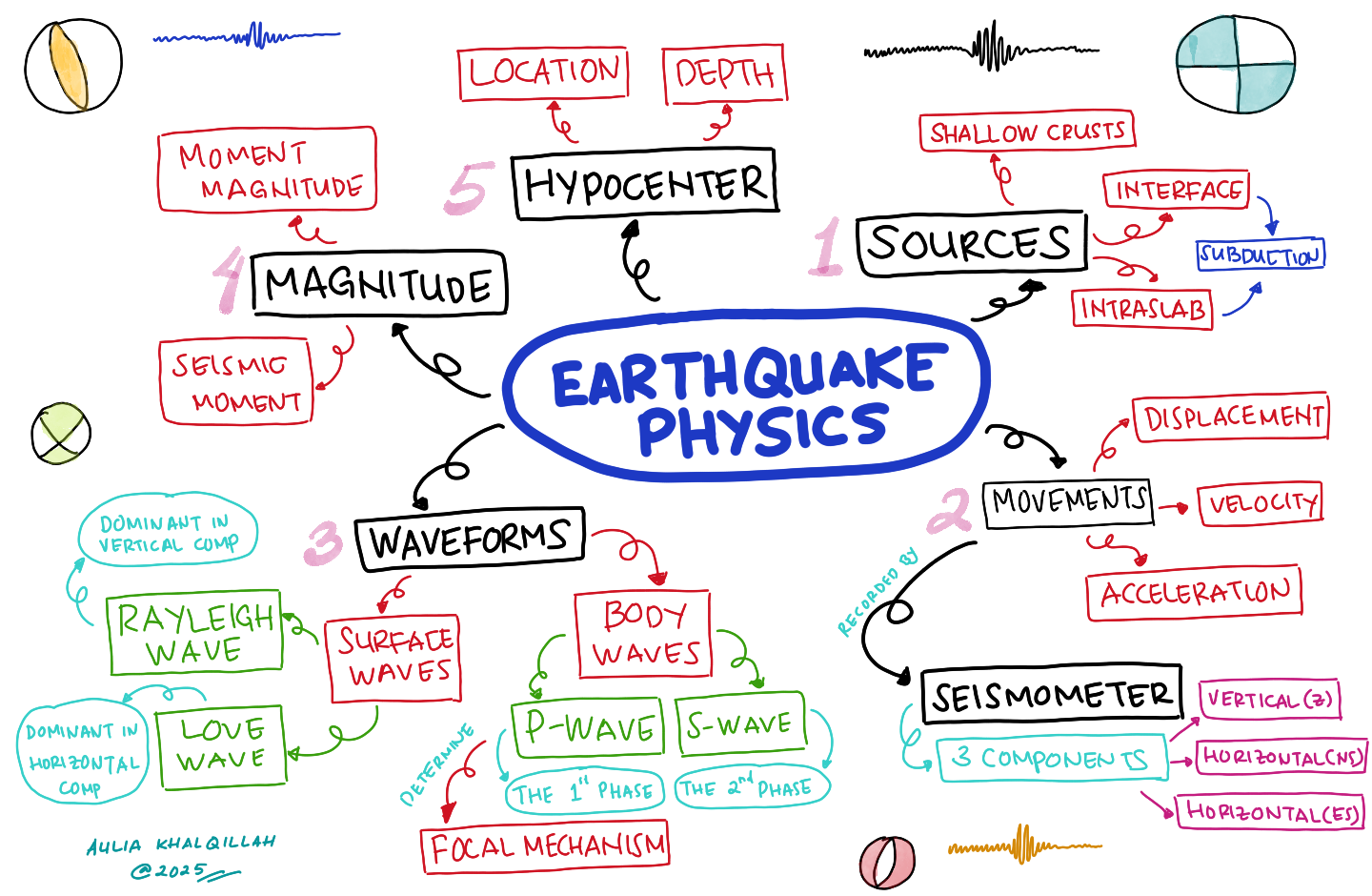
General topics in the earthquake physics

Earthquake physics is one of the physics’ topic branches. This scope explains how earthquakes can occur and what are the parameters and factors that can be accounted for by this process from the perspective of physics. Here, I will deliver the general information in terms of what can be learned from earthquake physics. By this end, you will obtain the understanding of

What are the main sources of the earthquake?
How do they move?
How to record the earthquake movement or related to it?
What is the visualisation of the earthquake record?
What is the quantity of the earthquake size and how to calculate it?
How to locate the earthquake location and its depth?

In my opinion, these topics are the keys to explain the earthquake framework.

Sources#

Earth has a complex structure that consists of multiple layers, crust, mantle, and core are the main compositions as shown in Figure 1. The crust is the top solid layer of earth, about 100 Km deep. This layer is divided into two types, the continental crust and the ocean crust. The continental crust’s thickness is about 7 Km and 40 Km - 100 Km for the ocean cruts. The ocean crust is denser than the continental crust.

The mantle layer is composed of magnesium and iron. About 80% of the earth’s layer is composed of the mantle layer where the depth is up to 2900 Km. The mantle layer is divided into two sublayers, upper mantle and lower mantle. The upper mantle is called Lithosphere which is composed of bulk materials, approximately 100 Km thick. The lower mantle is called Asthenosphere which is composed of non-rigid, weak, and high temperature material. The thickness of the Asthenosphere is approximately about 700 Km. The transition zone between Lithosphere and Asthenosphere is the weak zone and both layers can separate mechanically. Since the Asthenosphere is semi-fluid, it can flow slowly and make a movement of the material above it. This means that the Listhosphere moves over the Asthesnosphere. The implication of this process is the tectonic plates which move relative to each other and in certain time, it may generate collisions between plate boundaries, that is why the earthquake can occur. We will explain more.

earthlayer

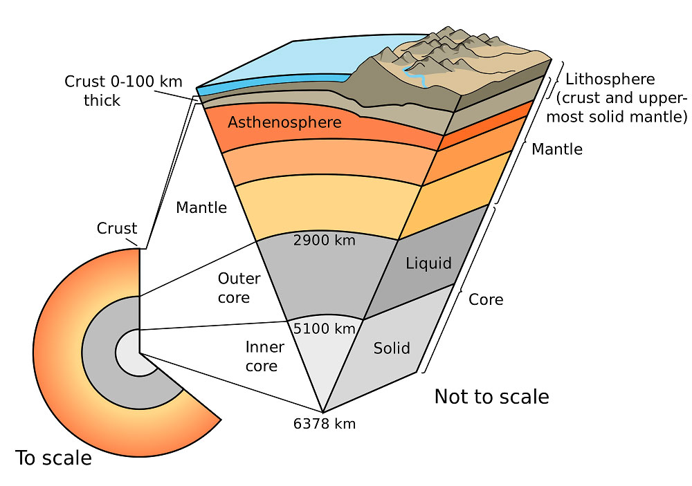
Figure 1. Earth structure layers (USGS)

The core layer is the deepest earth’s structure layer, about 6371 Km deep. The core is divided into two zones, outer core, and inner core. The silicon, iron-nickel, sulphur, and less oxygen are the compositions in the core layers. The outer core is the liquid layer that has the thickness of 2270 Km and can produce the electromagnetic field. The inner core is the higher temperature of the earth’s structure layer where the radius is about 1216 Km. The iron is mainly composed of this layer and it is solid even though the temperature is high because of the high pressure around the core. The heat from the core generates convection currents in the mantle, this process makes Asthenosphere drive Lithosphere.

Based on the MORVEL model, the global plate motion, there are 25 global plates that move to each other at varying velocity from 10 mm/yr to 100 mm/yr, depending on the plate zone. The earthquake occurs along these boundaries and it can be distinguished by three source zones: shallow crust, interface, and intraslab. The shallow crust earthquake occurs by the depth of less than 40 Km on the land. It can be represented as the faults, such as Sumatran Faults and others in Indonesia. The interface earthquake occurs in the interface between two plates by depth of 20 Km - 50 Km, then it is called a subduction zone where the low-density plate will drive under the high-density plate. The intraslab is also part of the subduction zone as well, however the earthquake depth will be found at deeper than 50 Km. The earthquake energy from intraslab is smaller than the interface and shallow crust sources because the energy has been attenuated by the distance and depth.

Movements#

The tectonic plates move relative to each other and can generate an earthquake in terms of vibration and it is visualised by a waveform. The vibration of an earthquake spreads from an earthquake source in a certain depth to any direction and it will reach the earth surface. This can be recorded by using a seismometer to quantify the physical parameters in terms of displacement, velocity, and acceleration. The explanation about seismometers will be discussed in the next subchapter. These parameters are the main key to explain the physical behaviour of an earthquake or ground motion in terms of seismic hazard.

The displacement measures how far an earth structure (rock or soil) deforms from its initial position to final position. The velocity measures how fast an earth structure moves in certain displacement relative to duration (time). The acceleration measures how much a rate of change of the velocity of an earth structure relative to duration (time). These parameters are extracted from the waveform. Specifically, earthquakes have their own waveform pattern. The topic of waveform will be explained in the next subchapter.

The simple mathematics approach for displacement (u), velocity (v) and acceleration (a) can be written in terms of harmonic wave as follows

u(x,t)= A sin (ωt±kx)

v(x,t)= ωA cos (ωt±kx)

a(x,t)= -2A sin (ωt±kx)

where the A is the amplitude of wave, is the angular frequency, ω=2πf, k is the wavenumber, k=v=2π, t is time in second, and x is the position. Based on these equations, the movement of earth structure has the variation of the frequency and velocity. Because the earth structure is complex, the waveform from the subsurface of the earth will fluctuate over the time and different over the position as shown in Figure 2.

eq_waveform

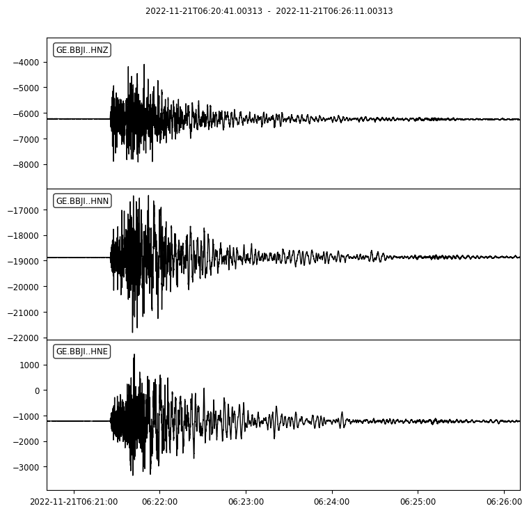
Figure 2. An example raw data of earthquake waveform of Cianjur’s earthquake in 2022-11-21 13:21:11 WIB. The waveform is downloaded from GFZ earthquake repository via Obspy (Python package).

In actuality, the earthquake waveform is shown in Figure 2. This is the earthquake waveform of Cianjur’s earthquake, Jawa Barat in 2022-11-21 13:21:11 WIB with moment magnitude of 5.5 and depth of 10 Km. This is the raw signal of the earthquake waveform that has been recorded in datalogger. The channels are HNE, HNN, and HNZ where the H code is high gain seismometer, N code is accelerometer, E code is for east component, N code is for north component, and Z code is for vertical component. The y-axis is the amplitude (in count), not yet in actual physical unit in terms of displacement, velocity or acceleration). To do that, we should conduct further processing, we call it a remove response to get the actual physical unit. This process will be explained in another article.

Seismometer#

A seismometer is a sensor to record a seismic wave either generated by an earthquake or ambient noise from the vibration beneath the earth surfaces. It is installed about 50 cm to 1 m relatively below the ground surface for earthquake waveform data recording. In case only for seismic ambient noise data recording, the seismometer is deployed on the ground surface for a short period of time. The seismometer has three components or channels, North-South (NS, horizontal 1), East-West (EW horizontal 2), and Vertical (Z). The sensor is very sensitive to any vibration sources and it has their own characteristics based on the objective which will be observed to. The types of sensors and its characteristics are resumed in the Table below.

Sensor Type	Frequency Range (Hz)	Application
Broadband	0.01-100	Detecting global earthquake
Short-Period	1-100	Detecting local earthquake
Long-Period	0.001-1	Study of low earthquakes, tectonic deformation
Accelerometer (Strong Motion)	0.1-50	Engineering seismology, structural response

In detail, the sensors have their own response file which contains detailed information about the sensor characteristics or parameters such as corner frequency, damping, and sensitivity. For more information you may find it here. The response file is used to get the original physical unit, such as displacement, velocity, and accelerometer through the remove instrument response process. The common sensor must be integrated to the datalogger. The datalogger is used to store the seismic wave in the raw format based on each datalogger type. Currently, there is a sensor that provides built-in datalogger (storage), such as Raspberry Shake and Nodes. The seismic wave data which is stored into the datalogger can be converted to the certain format (SAC, SEED, miniSEED, ASCII) for further waveform data processing.

Waveforms (Seismic Waves)#

In earthquake science, waveforms or seismic waves or earthquake waveforms (Figure 2) are divided into two types, Body Waves and Surface Waves. Body Waves consist of P-Wave and S-Wave. The P-Wave is the first main wave phase and travels faster than S-Wave, therefore S-Wave is the second main wave phase after the P-Wave in the earthquake waveform. The P-Wave can travel through the hard rock about Vp=5000 m/s and soft soil about Vp=1400-1500 m/s, while the S-Wave only travel in the solid layer about Vs=3000 m/s. The P-Wave is sensitive to the vertical component while the S-Wave is sensitive to the horizontal components as shown in figure below.

The first motion of P-Wave (Up-Compressional and Down-Dilatational) can be used to estimate a focal mechanism of an earthquake as shown in Figure 3. The focal mechanism represents the fault deformation form such as Strike-Slip, Normal, Reverse (Thrust), and Oblique as shown in figure below. These fault deformation forms are represented by parameters such as strike, dip, and rake. Strike is the fault plane direction from the reference of the north direction, if the strike is 90° which means the fault deforms in east-west direction. Dip is the angle between horizontal plane and fault plane. It is measured downward along the plane. The range of dip is 0° to 90°. Rake describes the angle between fault plane direction and slip of the plane. As I mentioned before, the focal mechanism is determined from the first motion or polarization of P-Wave from several earthquake waveforms which is obtained from several stations. The optimum focal mechanism is determined by the well distribution of seismic stations that cover an earthquake. We can access the focal mechanism that has been analysed by several agencies such as GFZ Earthquake Bulletin (you may find it with the MT abbreviation which stands for Momen Tensor) and Global CMT (GCMT).

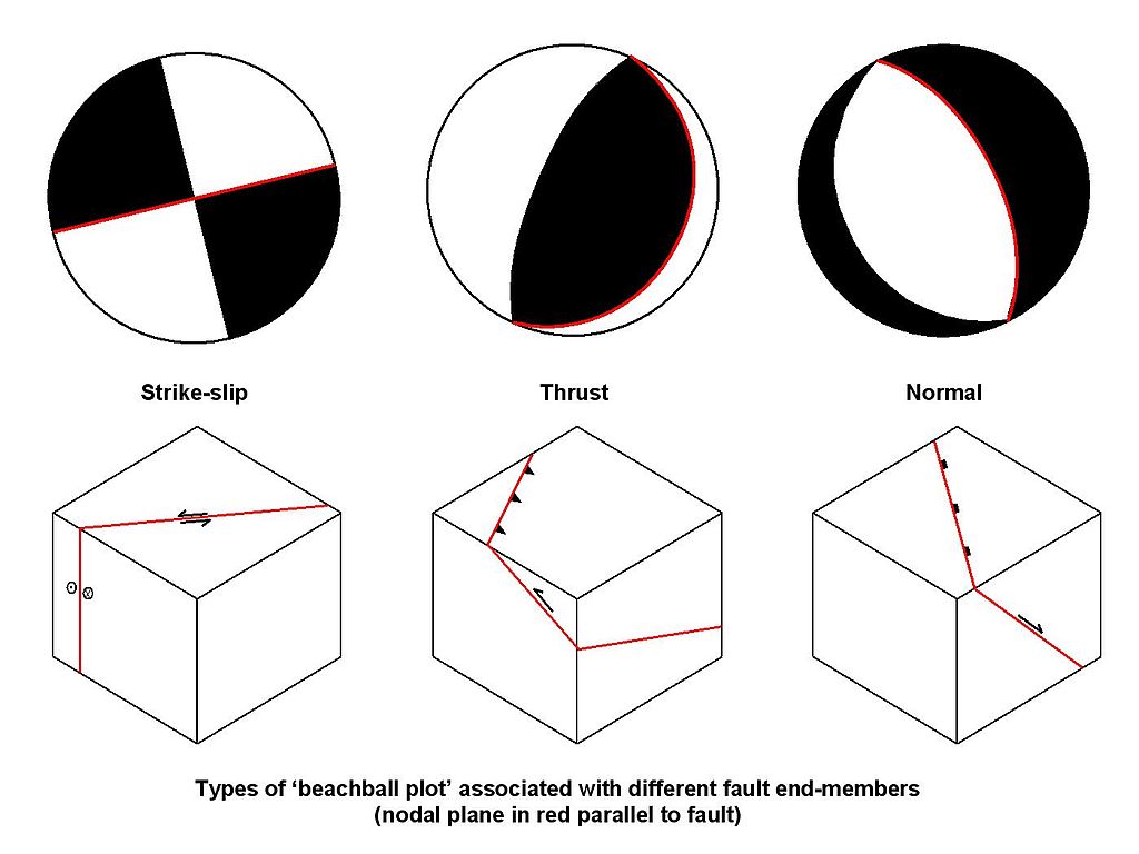
Figure 3. The types of focal mechanisms or beachballs

The main-second wave type is Surface Waves. The Surface Waves consist of Rayleigh Wave and Love Wave. The particle in Rayleigh Wave moves in elliptical motion and contributes to vertical and horizontal components, but much more sensitive to vertical components. The amplitude of Rayleigh Wave decreases with depth. The Love Wave, its particle moves horizontally on the surface caused by shear waves. That is why the Love Wave is more sensitive to horizontal components. The Love Wave can only travel to solid layers rather than liquid. The amplitude of Love Wave also decreases with depth. The Surface Waves can be used to evaluate the soil structure (below 30 m) through the flexible and rapid microtremor measurement. The parameter will be resumed by shear wave velocity below 30 m or Vs30. It is very useful for preliminary information of earthquake resistant building construction planning.

Magnitudes#

By using waveform data, we can extract other magnitude parameters besides Vs30. In advance, we can estimate the seismic moment (Mo) and moment magnitude (Mw). The Mw is the earthquake size that has been introduced by Hanks and Kanamori (1979) with a title “A Moment Magnitude Scale” and widely used to inform the public in this century. The Mw is determined by using Mo through the following equation

Mw=2/3 log10(Mo)-6

while the Mo can be estimated by using the following equation

Mo= A D

where the is the shear modulus of the rocks (pascals), A is the rupture area (square meters), and D is the average slip or average displacement of fault (in meters). The common average of shear modulus is around 30 GPa or equal to 3 x 10 10 Pa for crustal rocks. In detail, it depends on the geological condition of the region. The A and D can be estimated by using Well-Coppersmith’s empirical relationship (1994).

Hypocenter#

A hypocenter is the location and depth of an earthquake. The location is in longitude and latitude coordinates. The hypocenter is determined by waveforms from several stations; at least three stations record the earthquake waveforms. In detail, the arrival time of P-Wave and S-Wave are used to locate the earthquake position and its depth. By using the simple physics principle of straight line motion, d=v t, where d is distance in meter, v is velocity in m/s, and t is time in seconds, we then can locate them.

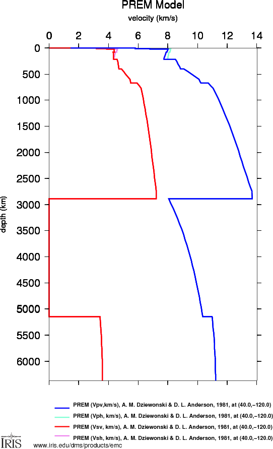
(a)	(b)

Figure 4. (a) PREM 1-D global velocity model and (b) an example of travel time of P-Wave and S-Wave (USGS)

Since we can calculate residual of arrival time between S-Wave and P-Wave (t) and velocity (we call it as velocity model, as shown in Figure above), we then can estimate an earthquake location based on distance of ray path d that travel beneath earth from the station. We can use several velocity models as initial velocity models either for 1D or 3D (tomography) velocity models such as PREM (Figure 4a), AK135, and etc (https://ds.iris.edu/spud/earthmodel). In order to estimate an earthquake depth (focal depth) Z, we can use the simple pythagoras approximation by using the distance of ray path d and surface distance between station and earthquake location (epicenter). The illustration can be seen in Figure 5.

eq_depth

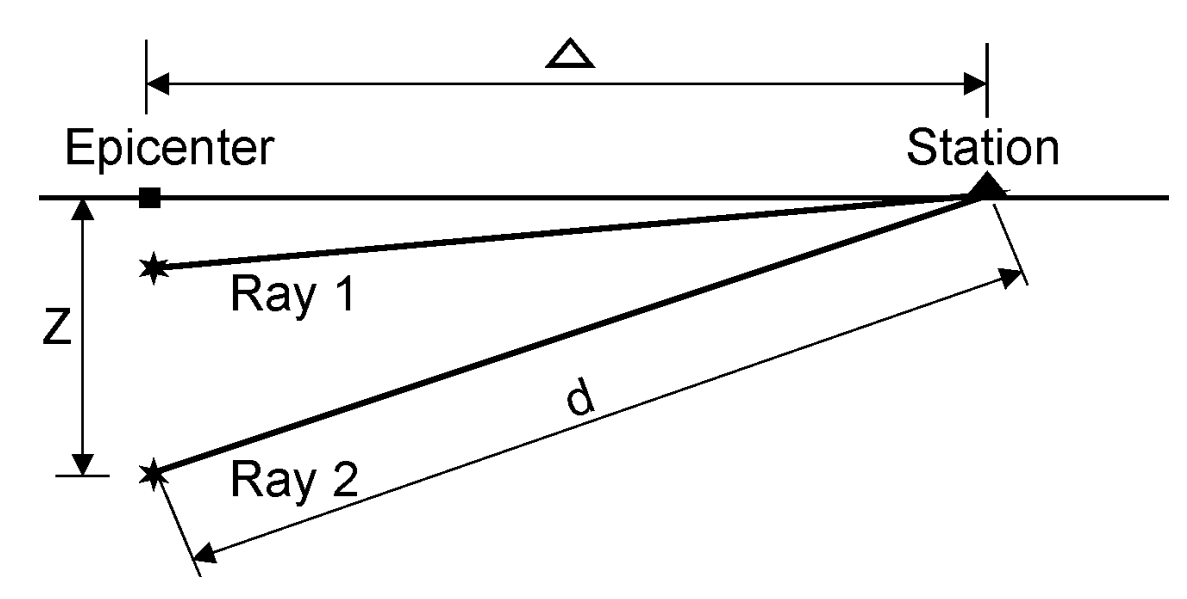
Figure 5. The illustration for estimate of focal depth schematic (Jens Havskov (2011))

In the simple mathematics form, it can be written as

Z^2= d^2 - delta^2$

This is a very simple approximation to estimate the hypocenter. We have to notice that the earth structures are not simple. We should use the advanced or complex algorithm approximation (numerical method) to obtain the earthquake structures information in more detail. Of course it still remains an uncertainty and limitation.